HCN Isomerization Reaction

This tutorial consists of several steps to study the isomerization reaction of HCN:

• Geometry optimization
• Linear transit
• Quick frequency calculation
• Transition state search
• Accurate frequency calculation
• IRC

Step 1: Prepare the HCN molecule

Start ADFjobs

Click on the Tutorial folder icon

Start ADFinput using the SCM → New Input menu command

Draw an HCN molecule (first the N, next the C and finally an H atom)

Select the C-N bond and make it a triple-bond

Pre-optimize the geometry

You should get a linear molecule:

Select the Geometry Optimization task

Select the DZP basis set

Select File → Run, give it the name HCN_GO

The geometry will be optimized, using a DZP basis set.

Click “Yes” when asked to read new coordinates from the HCN_GO.t21 file

Check the C-N and C-H distances

They should be about 115 and 108 pm (1.15 and 1.08 Angstrom), respectively.

Write down the value of the bonding energy printed

at the end of the calculation in the ADFtail window

Step 2: Create a rough approximation for the transition state geometry

The HCN molecule has an CNH isomer. There is an energy barrier between these two states. We are going to find the transition state and calculate its height.

To find a better starting point for the transition state search we will perform a linear transit calculation as a rough approximation of the reaction path. We will vary the H-C-N angle in steps between 40 and 140 degrees and let ADF optimize bond lengths at each angle.

To set up the linear transit calculation:

Select the Linear Transit task

Click on the button next to task to go to the ‘Geometry Constraints and Scan’ panel

Select all the atoms

You should see ‘+ N(1) C(2) H(3) (angle)’ note in the right panel now:

Click the ‘+’ button to add the angle constraint

Now ‘- N(1) C(2) H(3)’ and the two fields as limits for the degree parameter appear.

Enter ‘140’ and ‘40’ in the ‘degrees’ fields

ADF will have trouble running the current set up because the HCN molecule is perfectly linear. So we will help ADF by changing the angle to 140 degrees, the same as the first point of the LT scan.

Use the slider to change the HCN angle to 140 degrees

The set up is complete. Now we will run the LT calculation, but we will save it with a new name as we wish to keep the results of the HCN_GO calculation:

Use File → Save As to save the file as ‘HCN_LT’

Run the calculation

Running might take a few minutes. When the run is finished:

Click “Yes” when asked to read new coordinates

You will see the last geometry, close to CNH. To see how geometry was changing during the LT run, use ADFmovie:

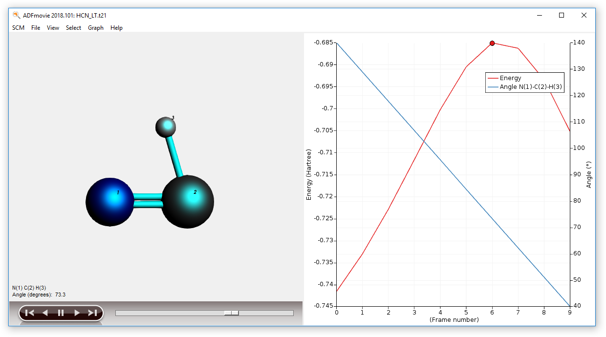
Select the SCM → Movie command

Select all atoms (use shift-drag to make a rectangle around the atoms)

Select the Graph → Distance, Angle, Dihedral command (to get the angle graph, as three atoms are still selected)

Use the View → Converged Geometries Only command

Zoom in to get a better view of the molecule

Press the Play button (the right-pointing triangle in the controls at the left bottom of the ADFmovie window)

You will see the hydrogen atom moving from C to N. You will also see a graph of the energy as function of the LT steps. As the movie is playing a dot shows the corresponding position in the graph.

Somewhere along the path, there is a transition state we are looking for. Remember that you needed to use the ‘Optimized Geometries Only’ command to filter out all the intermediate geometry step, so that you get only the converged geometries for each LT step.

In the graph, click (without moving!) on the top of the energy graph

Alternatively, use the arrow keys (cursor keys) to move between different steps, or use the slider

Check which geometry has the maximum energy

You should find that at around an angle of 60-75 degrees the maximum energy is reached. This is Frame 6 (the 7th LT step):

You can find this information also in the output file:

Select the SCM → Output menu command

In the ADFoutput window select the Other Properties → ‘LT Path command

You will see that indeed the geometry number 7 (corresponding to Frame 6 in ADFmovie) has the highest energy. In this particular example the choice of the angle is not very important, but in general you will always want to get the best approximation for the transition state available.

We will now prepare the search for the transition state starting from this geometry:

Click in the ADFmovie window

Make sure frame 6 is selected

Use the File → Update Geometry In Input command

The geometry of HCN in your ADFinput window will be updated to match the geometry currently selected in the ADFmovie window:

Step 3: Finding the transition state: prepare approximate Hessian

In general, it is important to have a good starting Hessian with one imaginary frequency when performing a TS search. We are going to create such a Hessian by doing a quick frequencies calculation:

Select the Frequencies task (from the Main panel)

Make sure the Numerical quality is set to Normal

Save the molecule as ‘HCN_Freq1’ (Save As)

Run the calculation

The frequency calculation is now in progress and will run very fast. When it has finished:

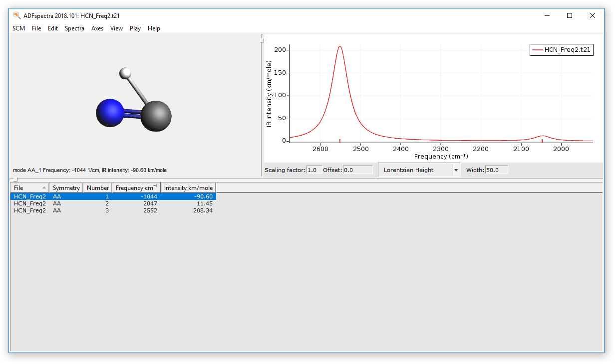
Select the SCM → Spectra command

If everything was done correctly, you should see a spectrum with two peaks in the range of 2000 - 3000 1/cm. In the table you can see three frequencies, two shown in the spectrum and one negative frequency (around -1000 1/cm). A negative frequency value actually means that it is an imaginary frequency.

Click with your mouse on the peak corresponding to the imaginary frequency

The normal mode corresponding to that frequency will show on the left side. Check that the frequency indeed corresponds to the H atom moving parallel to the C-N bond.

Step 4: Search for the transition state

The result file, HCN_Freq1.t21, has an initial geometry for our transition state search. It also contains a Hessian matrix (produced with the frequencies calculation) that can be used to kick-start the TS procedure.

Bring ADFinput with the HCN_Freq1 calculation to the foreground

Select the Transition State task

ctrl/cmd-F and search for ‘restart’, select the ‘Files (Restart)’ panel

Click the file select button (looks like a folder) in front of the empty ‘Restart file:’ field

Select the HCN_Freq1.t21 file and click ‘Open’:

Save the set up as HCN_TS (Save As)

Run the calculation

After the calculation has finished (again very fast), you will be asked to read the new geometry from the results file HCN_TS.t21:

Answer “Yes” to import the latest geometry

Make a note of the bond energy for the transition state (visible in the logfile)

ADFinput will now display the transition state geometry.

If you compare the bond energy with the bond energy of the optimized HCN molecule from the first calculation, the difference should be about 1.9 eV. Also check that the geometry makes sense: the C-H and C-N distances should be around 1.20 and 1.19 Angstrom and the H-C-N angle should be about 70 degrees.

Step 5: Calculating frequencies at the transition state

After every transition state search it is good practice to verify that you indeed have one and only one imaginary frequency. For this we will repeat the frequency calculation at the TS geometry:

Make sure you have HCN_TS open in ADFinput

Select the Frequencies task (from the ‘Main’ panel)

Save with name HCN_Freq2

Run

The calculation is running, should not take much time. After the calculation has finished:

Select the SCM → Spectra command

You will be presented with an IR spectrum of the molecule featuring two normal modes. In the table you should also see one negative frequency (corresponding to an imaginary frequency).

Click on the mode with negative frequency

The visualization of the normal mode corresponding to this frequency should make it clear that this is indeed the reaction coordinate we are studying.

Step 6: Following the reaction coordinate

ADF can follow the minimum-energy path from the transition state to one or the other product. The method used in ADF for this is called Intrinsic Reaction Coordinate (IRC). You may want to skip this part as the calculation might take some time to complete.

Bring HCN_Freq2 in ADFinput to the front

Select the IRC task

Go to the ‘Intrinsic Reaction Coordinate (IRC)’ panel (in Model, or via the search, or by clicking on the button)

This panel allows you to specify various parameters for the IRC method. The most important parameter is the direction to follow. The choice is more or less arbitrary. By choosing “Forward path” or “Backward path” will lead you to one or the other product but it’s hard to tell which of the two in what case. We will calculate both paths at once, so we do not need to change the default.

Another option is the ‘Rerun IRC points’. When checked, after the IRC calculation has finished an extra single point calculation will be performed for each converged points, and the results will be saved. This will allow you to observe in more detail what happens along the IRC path, for example how orbitals change. In this tutorial, lets show how this work, so turn that feature on:

Check the ‘Rerun IRC points’ checkbox

Tip

The ‘Rerun IRC points’ option also works with Fragment analysis:

- check the Fragment Analysis tutorial

- define fragments via Regions (see Fragments tutorial)

- check the ‘Use fragments’ check box on the MultiLevel Fragments panel

We also want to make sure all optimizations converge, so lets increase the maximum number of iterations to 50. And as IRC needs a good Hessian, restart the calculation from the Hessian calculated in the TS:

Click on the after Convergence details

In the Number of geometry iterations field specify 50

Go to the Files (Restart) panel in the Details section, and select the HCN_Freq2.t21 result file as Restart File

Save as HCN_IRC

Run

After some minutes the calculation will finish. You can use ADFmovie to view the IRC path. Of course you need again to make sure to show the converged geometries only:

Select the SCM → Movie command

Select the View → Converged Geometries Only command

Click OK when the warning message appears (about the changed order of steps)

Select all atoms

Select the Graph → Distance, Angle, Dihedral command

From this movie you can see the IRC path, and the energies at the most interesting points. As we have calculated the forward and backward path in one run, the order of the forward path needs to be reversed to get a proper energy graph.

You can also examine some properties along the IRC path by studying the output file:

Select SCM → Output

Use the Other Properties → IRC Path menu command

You will see a table with the properties along the forward path. To get the backwards path:

Click on the blue header ‘Dist from TS ...’

The output browser should jump to the next section with that header, which is the table for the backward IRC path.

Step 7: Following orbitals along the IRC: reporting from .t21 files

In the previous IRC calculation you had activated the Rerun IRC points option. As a result the data for all the converged IRC points is also available.

Bring ADFjobs to the foreground

Click on the triangle for the HCN_IRC job to see the job files

If you wish you can select the .t21 file of interest, and use the GUI tools (ADFview, ADFlevels, KFBrowser) to examine the results for that particular IRC point in detail. You can also use the Report tool to generate an overview:

Job → Open .results to open the .results in ADFjobs

Select all sp_... jobs (click on the first, shift click on the last)

Tools → Build Standard Report

Save the job with a name like ‘HCN IRC results’

Wait until the report generation is ready,

the ADFjobs status line at the top will give an indication of the progress

Now you should have a nice overview of the detailed results, as set up in the report options, for all of the IRC points:

Another example of using the Report tool can be found in NH3 Basis Set tutorial.

Step 8: Following orbitals for the LT afterwards: generating jobs for many geometries

For Linear Transit runs you also might want to follow orbitals, or check other properties for the converged points. You can do this in exactly the same way as for the IRC run (thus, by activating the Rerun LT points option). However, this option was not activated.

There is an easy way to generate the information for the converged points afterwards as well. Note that this would also work after an IRC calculation instead of a LT calculation.

Activate ADFjobs

Select the HCN_LT job

Tools → Prepare

In the Prepare window that appears:

In the “Use coordinates from” section, press the “+” and select “ADF result file()s (.t21)”

Select the HCN_LT.t21 results file, and click Open

In the “Use the input options section”, press the “+” and select “Run Type → SinglePoint”

Click OK

Select all the SP.HCN jobs that have been generated

Job → Run

Wait for the calculations to finish

Now we can use the Report Tool to generate an overview, just as we just did for the IRC calculations:

Select all SP.HCN_LT...jobs (click on the first, shift click on the last)

Tools → Build Standard Report

Save the job with a name like ‘HCN LT results’

Wait until the report generation is ready,

the ADFjobs status line at the top will give an indication of the progress

Now you should have a nice overview of the detailed results, as set up in the report options, for all of the LT points:

Finally, at the end of this tutorial you will have many open windows. To close all ADF-GUI related windows at once, you may use the SCM → Quit All command.