Electronic transport with DFTB-NEGF

In this series of tutorials we will show how to model coherent electron transport using DFTB-NEGF.

We advise to go through the following tutorials in the order they are presented.

See also

DFTB-NEGF documentation

Carbon nanotube

Let us begin by modeling the electron transport through a carbon nanotube:

Setting up the system

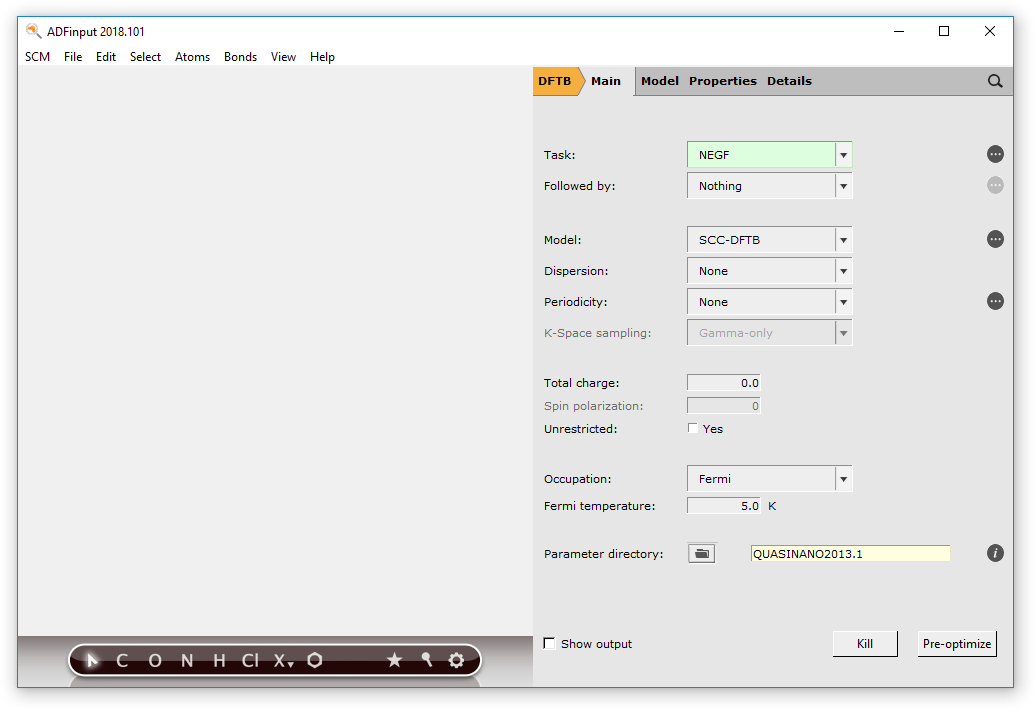
Start up ADFInput

1. Switch to DFTB

2. Select Task → NEGF

3. In the Main DFTB panel click on Parameter directory → QUASINANO2013.1

4. Click on to switch to the NEGF panel (or click on Model → NEGF)

From the NEGF panel we can set up the geometry of our system and specify various NEGF calculation parameters:

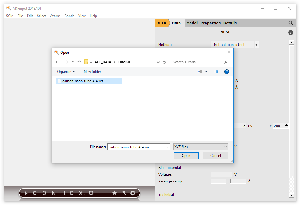
We first need an .xyz file defining our lead, that is, a carbon nanotube:

Click here to download the .xyz file carbon_nano_tube_4-4.xyz

We now import our lead:

1. Click on the folder icon next to Lead: this will prompt a file dialog window

2. Open carbon_nano_tube_4-4.xyz (the .xyz file you just downloaded)

This will import the left and right leads. Now set the number of lead repetitions to 2:

Set Lead Repetitions to 2

Note

The leads cannot be directly modified in the molecule-editing area. In the next tutorial we will show how to create a lead.

We now need to define our central region. In this tutorial, the central region consist of a nanotube (same as in the lead). We can easily fill in the central region with lead-material with the Fill central region option:

1. Click on Fill

2. Enter 2 in the prompted dialog window and click on OK

This concludes the geometry-building part of a NEGF calculation. Your system should look like this:

Running the calculation

From the NEGF panel we can change other NEGF parameters, but in this tutorial we will use the default values.

We are ready to run the calculation:

Click on File → Save as...

Run the calculation with File → Run

Wait for the calculation to finish

Visualizing the results

The results can be visualized with ADFSpectra. To start up ADFSpectra:

Click on SCM → Spectra...

Here you can visualize:

• Transmission function \(T(E)\)
• NEGF-DOS (density of states)
• Current v.s. Bias Potential (computed from the the zero-bias Transmission function)

In ADFSpectra, click on Spectra → Transmission / Transmission+DOS / Current

Note

Energies are relative to the Fermi energy of the lead, i.e in the picture below, 0 eV corresponds to the Fermi energy of the nanotube (first simulation in Simulations work flow)

This is the transmission function of our nanotube:

and the Current v.s. Bias Potential characteristic:

CO on 1D gold chain

Introduction

This tutorial is inspired by Electronic and Transport Properties of Artificial Gold Chains PhysRevLett.93.096404 and Benchmark density functional theory calculations for nano-scale conductance The Journal of Chemical Physics 128, 114714 (2016).

We will study the electronic transport through an atomic gold chain, and study the effect that an adsorbed CO molecule has on the conductance.

According to PhysRevLett.93.096404 “a single CO group [...] modulates the electronic wave functions, acting as a ‘‘chemical scissor’’ along the gold chain, to strongly modify the coherent transport properties of the system”.

Creating the lead file

Let’s begin by creating a lead file. A lead file is a simple .xyz file with an extra lattice vector.

Tip

The folder $ADFHOME/atomicdata/Molecules/NEGF/Leads contains some pre-defined lead files

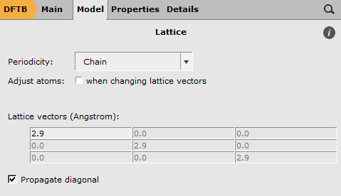
For this tutorial the lead will be a single gold atom with a lattice of 2.9 Å (in the x-direction). Let us create this with ADFInput:

Start up ADFInput

1. Switch to DFTB

2. From the main DFTB-panel, select Periodicity → Chain

3. Click Click on to switch the Lattice panel

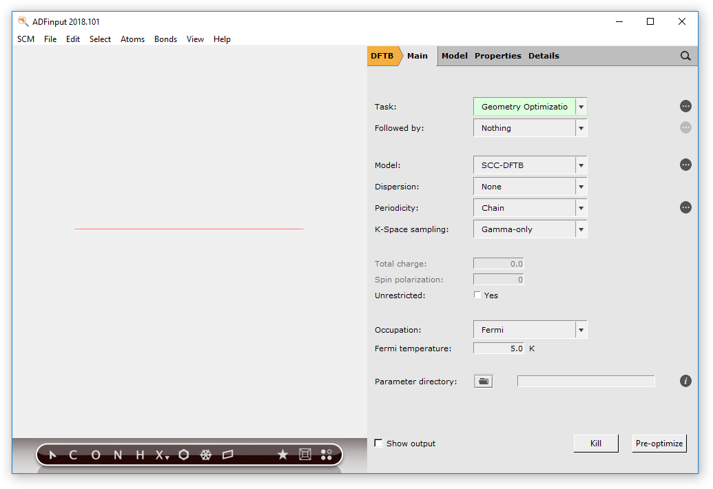
In the lattice panel we can specify the lattice vector:

Set the lattice vector to 2.9

We now add the gold atom

1. Click on ‘X’

2. Select ‘Au’

3. Click anywhere in the drawing area to add the gold atom

and set the coordinates of the gold atom to (0,0,0):

1. Click on Model → Coordinates

2. Set the xyz coordinates on the Au atom to (0,0,0)

We now export this 1D gold chain as an .xyz file:

Click on File → Export Coordinates...

Save the file as “Au_lead.xyz”

Close ADFInput File → Close

The .xyz file, defining our lead, should look like this:

1

Au       0.00000000       0.00000000       0.00000000
VEC1     2.90000000       0.00000000       0.00000000

Gold chain transport calculation

We are now ready to set up the DFTB-NEGF gold chain calculation:

Start up a new ADFInput (SCM → New Input)

1. Switch to DFTB

2. Select Task → NEGF

3. In the main DFTB panel click on Parameter directory → QUASINANO2013.1

4. Click on to go to the NEGF panel (or click on Model → NEGF)

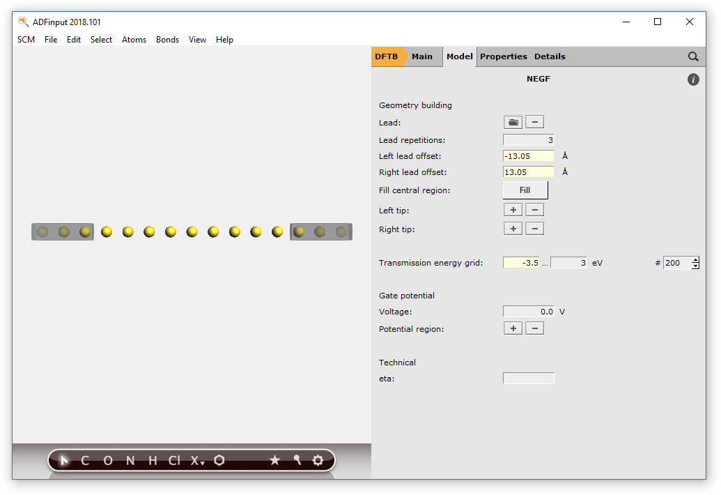
Import the lead file we just created (‘Au_lead.xyz’):

Click on the folder icon next to Lead: this will prompt a file dialog window

Open Au_lead.xyz (the .xyz file you just created)

Fill the central region with 9 gold atoms using the “Fill central region” option:

Click on Fill

Enter 9 in the prompted dialog window and click on OK

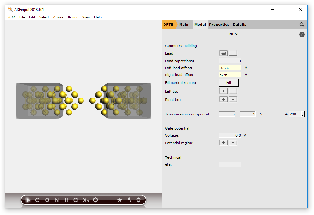
Let us also change the range for the Transmission energy grid to [-3.5,3.0], to match the energy range of PhysRevLett.93.096404:

Set the Transmission energy grid from -3.5 to 3.0

This is what your set-up should look like:

We are now ready to run the calculation and visualize the results with ADFSpectra:

Click on File → Save as...

Run the calculation with File → Run

Wait for the calculation to finish

Click on SCM → Spectra...

This is the computed transmission function through a 1D gold chain:

CO on gold chain transport calculation

We now modify our previous system by adding a CO molecule in the central region:

Select the ADFInput window: SCM → Input

Add the CO molecule by copy-pasting the following coordinates into ADFInput (CTRL+V in molecule drawing area)

O     0.0   0.0   3.12
C     0.0   0.0   1.96

The gold atom on which CO is adsorbed is “pulled” towards the CO molecule by 0.2 Angstrom:

In the Coordinates panel adjust the position of the central gold atom to (0.0, 0.0, 0.2)

Your system should look like this:

Tip

It is good practice to include some buffer lead material in the central region, and test the convergence of the results with respect to the size of this buffer (in this tutorial we have 4 buffer gold atoms on each side of the central Au-CO).

Run the calculation and visualize the results with ADFSpectra:

Click on File → Save

Run the calculation with File → Run

Wait for the calculation to finish

Click on SCM → Spectra...

This is the computed transmission function when CO is adsorbed on a gold chain.

As expected, the conductivity around the Fermi energy is “suppressed” by the adsorbed CO molecule.

Au-(4,4’-bipyridine)-Au molecular junction

In this tutorial we will use the NEGF geometry building tools to create a Au-(4,4’-bipyridine)-Au molecular junction:

Using tips

Start up ADFInput

Switch to DFTB

Select Task → NEGF

In the main DFTB panel click on Parameter directory → QUASINANO2013.1

Click on to go to the NEGF panel (or click on Model → NEGF)

Import the leads and fill the central region with 4 layers of lead material:

Click here to download the lead file Au3x3_lead.xyz

Import the lead file Au3x3_lead.xyz by clicking on the folder icon next to Lead

Fill the central region with 4 layers of lead material

We now carve two tips out of the central gold wire:

Select the gold atoms as shown in the picture below

Delete the selected atoms by pressing delete on your keyboard

We need to make space in the central region for the 4,4’-bipyridine molecule; to this aim we define a left tip and a right tip:

1. Select the gold atoms on the left-hand side

2. Click on + next to Left Tip in the NEGF panel

Clear the selection by clicking anywhere in the molecule-drawing area

3. Select the gold atoms on the right-hand side

4. Click on + next to Right Tip in the NEGF panel

Your system should now look like this:

Tip

You can remove atoms from a tip by selecting them and clicking on - next to Left/Right Tip in the NEGF panel

The tips are now anchored to their respective leads. If we move the two leads via the Left/Right lead offset, the tips will follow them.

Make space for 4,4’-bipyridine molecule:

Set the Left lead offset to -10.0 Angstrom

Set the Right lead offset to 10.0 Angstrom

and import it:

Click here to download the .xyz file 4_4_bipyridine.xyz

Click on File → Import Coordinates

Open 4_4_bipyridine.xyz (the .xyz file you just downloaded)

Your system should now look like this:

Tip

It is good practice to test the convergence of the results with respect to the number of lead repetitions and and amount of buffer lead material in the central region

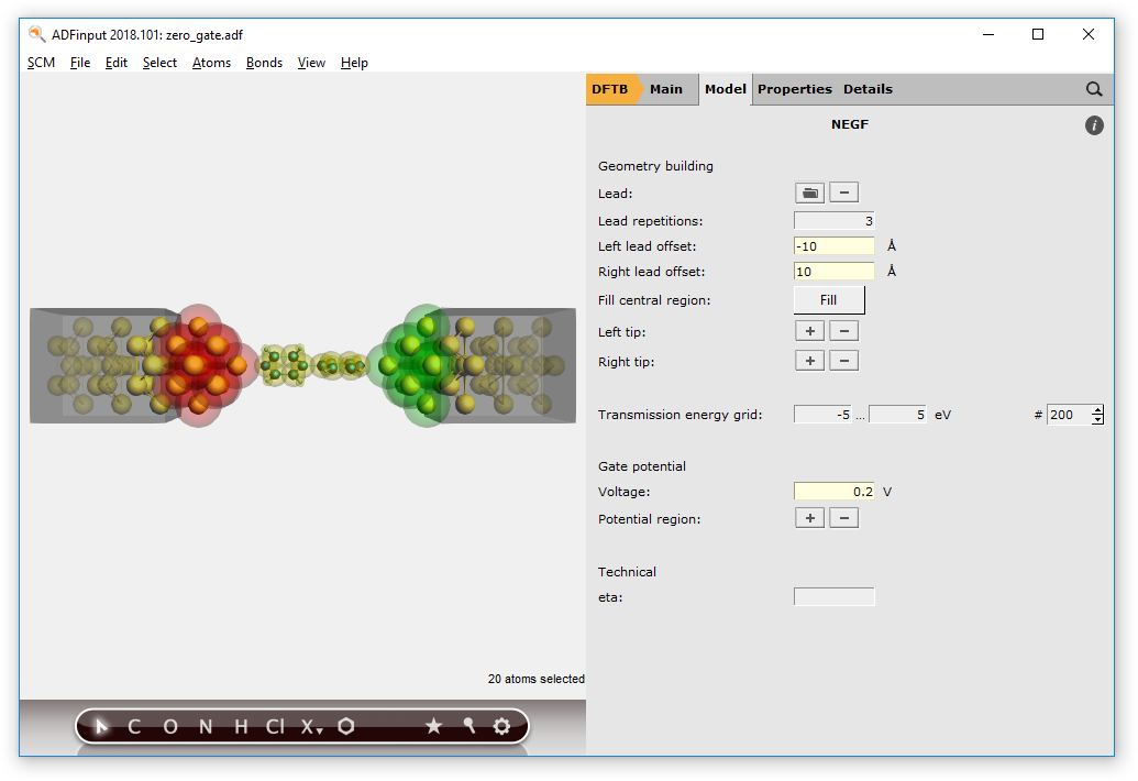
We are now ready to run the calculation:

Click on File → Save, and name the job “zero_gate”

Run the calculation with File → Run

Wait for the calculation to finish

Gate potential

To include a gate potential for the 4,4’-bipyridine molecule:

In the NEGF panel in ADFInput

1. Select the 4,4’-bipyridine molecule

2. Click on + next to Gate potential region in the NEGF panel

3. Set the Gate Voltage to 0.2 V

We will now run the job and visualize the results:

Click on File → Save as... and save it as gate_0.2

Run the calculation with File → Run

Wait for the calculation to finish

Click on SCM → Spectra...

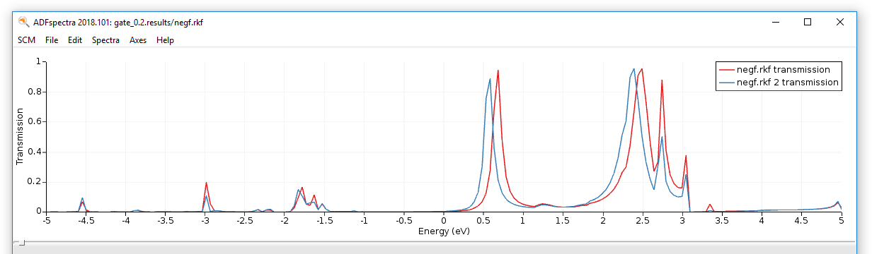
To better see the effect of the bias potential on the transmission function, we can add the transmission functions at zero gate we computed earlier:

In ADFSpectra click on File → Add and select negf.rkf in the gate_0.2.results folder