NiO and DFT+U¶

This tutorial will show you how to:

perform a single point calculation including the DFT+U formalism using the BAND-GUI

Step 1: adfinput¶

Start ADFinput in a clean directory. (according to Step 1 of the Getting Started with BAND)

Step 2: Setup the system - NiO¶

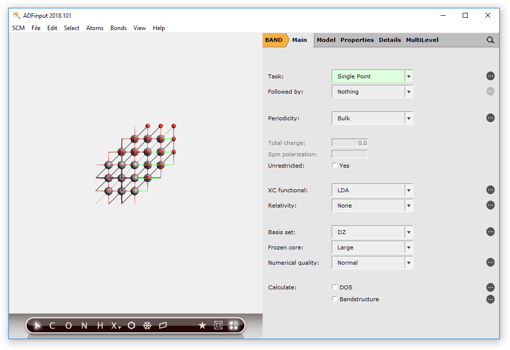
You can copy-paste the following information into the GUI directly.

2

Ni    0.000  0.000  0.000
O     2.085  2.085  2.085
VEC1  0.000  2.085  2.085
VEC2  2.085  0.000  2.085
VEC3  2.085  2.085  0.000

Step 3: BP86 without Hubbard¶

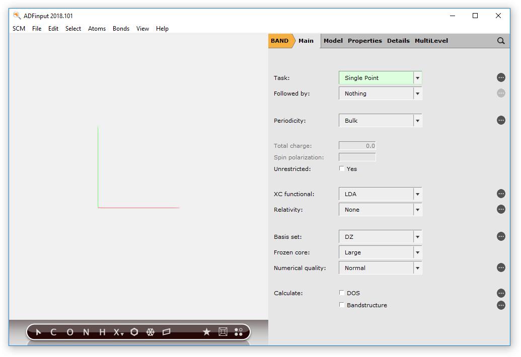
Go to the Main panel for BAND,

: 1. Panel bar Main

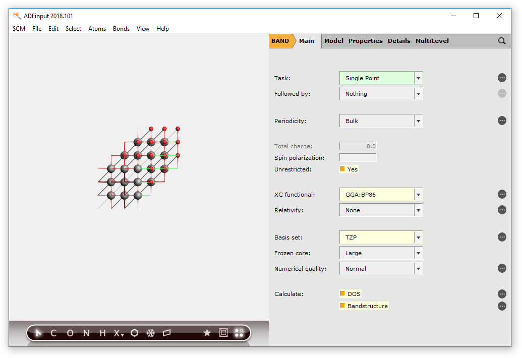
and change the calculation setup (XC functional, basis set) according to the following picture.

: 2. Check the Unrestricted box.

3. Set XC functional to GGA:BP86.

4. Set Basis Set to TZP

5. Tick the checkbox DOS

Step 3a: Run the calculation¶

Now you can save and run the calculation.

: File → Save, give it a name and press Save.

File → Run

Step 3b: Checking the results¶

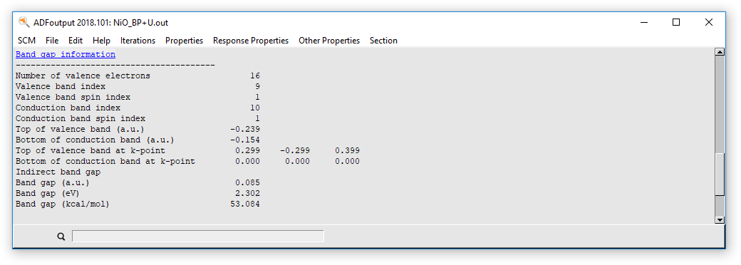
After the calculation finished, you can check the Output for the ‘Band Gap Info’.

: SCM → Output

Properties → Band Gap Info

One can see that there is no band gap at all. This contradicts experimental studies, which predict values between 3.7 to 4.3 eV.

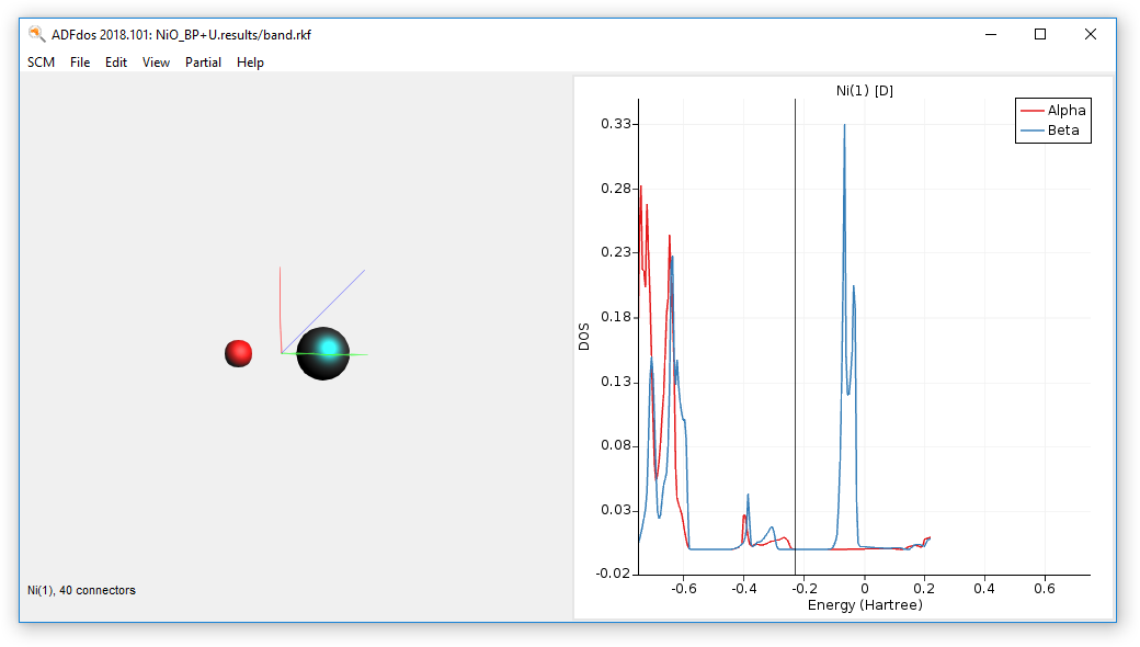
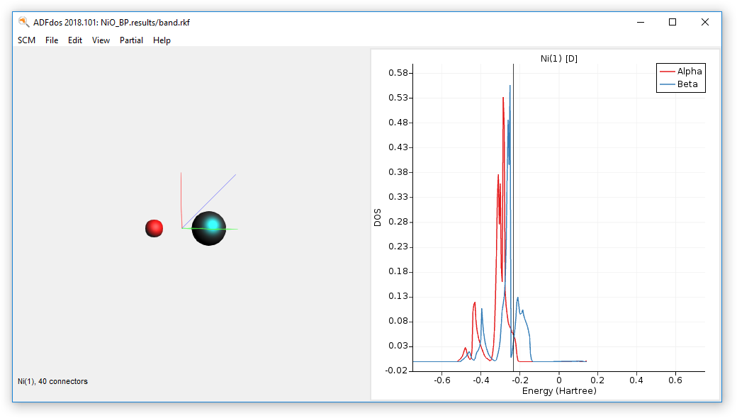
Plotting and examining the partial density of states (pDOS) for this calculation reveals that the d-orbital contributions of Ni are crossing the Fermi level.

: SCM → DOS

Select the Ni atom.

Choose Partial → Ni(1) → D-DOS

Step 4: Run the calculation - BP86+U¶

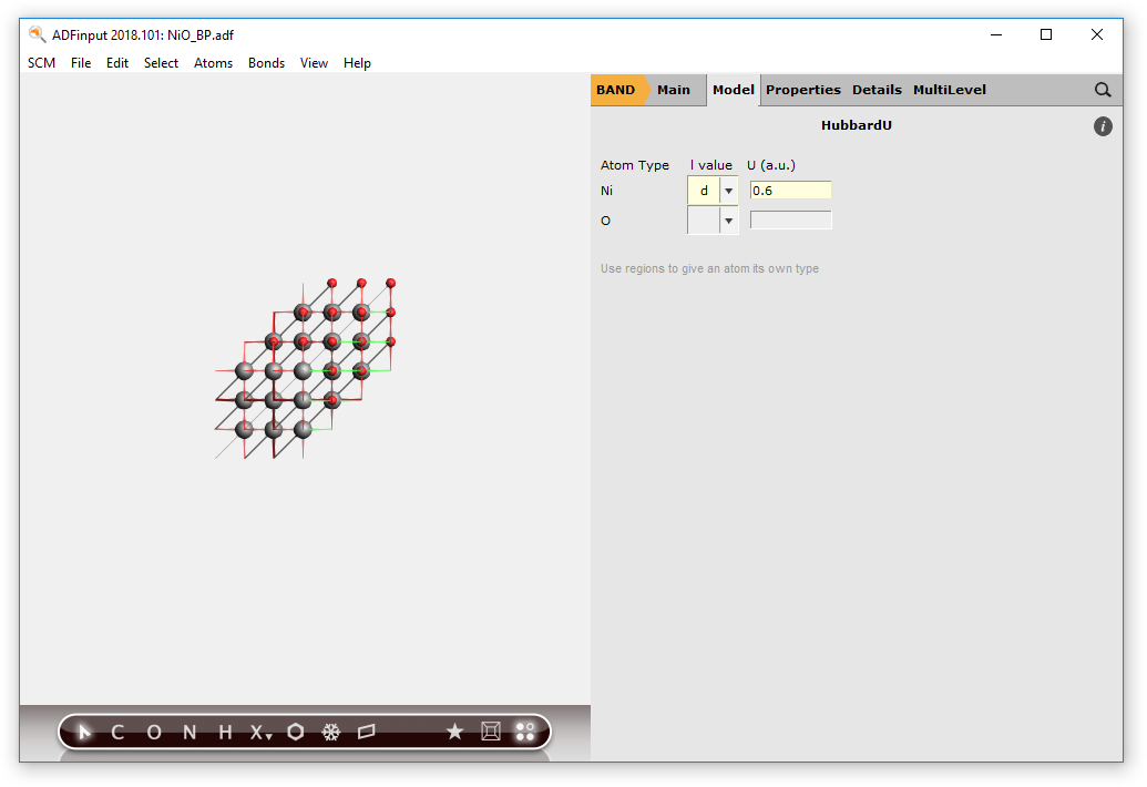
Go back to the Main menu of adfinput, change to HubbardU menu, and apply an U value of 0.6 a.u. to the d-orbitals of the Ni atom.

: Go to Model → HubbardU.

Set for Ni the l-value to d and the U value to 0.6.

This will influence the Hamiltonian and results in a state which tries to omit partial occupation or degeneracy w.r.t. the d-orbitals.

Step 4a: Run the calculation¶

Now you can save and run the calculation.

: File → Save, give it a name and press Save.

File → Run

Step 4b: Checking the results¶

After the calculation finished, you can check the Output for the ‘Band Gap Info’.

: SCM → Output

Properties → Band Gap Info

One can see that there is now a band gap of 2.3 eV. This is still less than the experimental values. That can be traced back to the neglection of the correct magnetic behavior of NiO.

Plotting and examining the partial density of states (pDOS) for this calculation reveals that the d-orbital contributions of Ni are no longer crossing the Fermi level.

: SCM → DOS

Select the Ni atom.

Choose Partial → Ni(1) → D-DOS