Multiple molecules, conformers, multiple methods

The ADF-GUI can handle multiple molecules, or multiple methods, or both, with one relatively simple setup. It also can generate and handle conformers. The handling of the conformers is actually an example of handling multiple molecules at once.

Multiple molecules

With ADFinput you can set up a calculation, and then run your set up for multiple molecules automatically. At run time the molecules are then taken from an .sdf file that has the same name as your .adf file (except for the extension obviously). This SDF file may come from somewhere else, from a Conformer-generation job for example, or you can actually create and edit multiple molecules inside ADFinput.

After the calculation the result is a new .sdf file. That .sdf file is a standard SDF file, with the calculated energy in the title for each molecule. It also contains references to the calculation results for the individual molecules. And it may contain some extra information per molecule (depending on the calculation).

As an example, let’s calculate the H-NMR spectra for methane and ethane with one single set-up.

Step 1: Set up methane and ethane in ADFinput

Start ADFinput

Create methane

Next we will add an extra molecule (ethane) to ADFinput:

Use the Edit → New Molecule menu command

Create ethane

Switch between the two molecules using the tabs at the bottom

Adjust the names of the tabs to methane and ethane (click on the name, it becomes editable)

When you would make many molecules the tabs will be replaced by a slider which you can use to run through your molecules.

Step 2: H-NMR calculation

Next we will set up the calculation of an H-NMR:

Go to the NMR panel (in the Properties section)

Check the Shielding for all H atoms check box

Use the File → Run menu, save your job as NMR

When asked to run all 2 molecules, click Yes

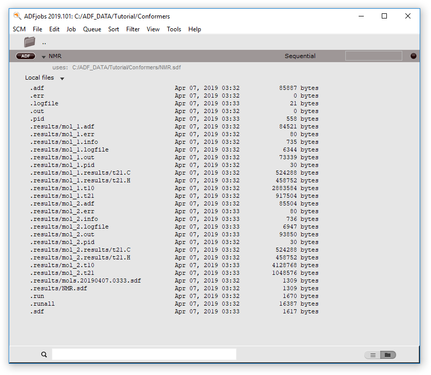
In the ADFjobs window you should see the job running. Also note that it gives you the information that the job uses the nmr.sdf file. When you open the job you will see the results for two different molecules in the .results folder:

Wait for the calculation to finish

Click on the triangle before the job name to see the files belonging to that job

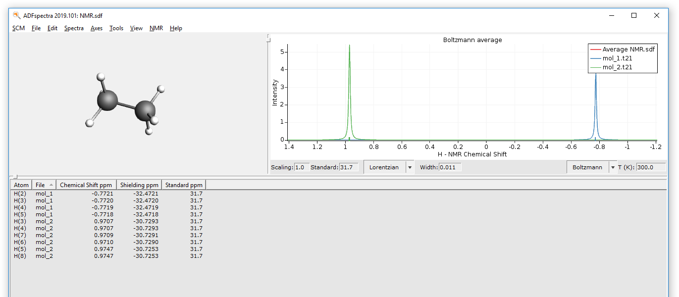
Use ADFspectra to see the calculated NMR spectra. When opening the job, it will show an averaged spectrum. Use the View menu to adjust what curves to see:

SCM → Spectra

In the ADFspectra window: View → Average/All Curve

Change the width of peaks to 0.01

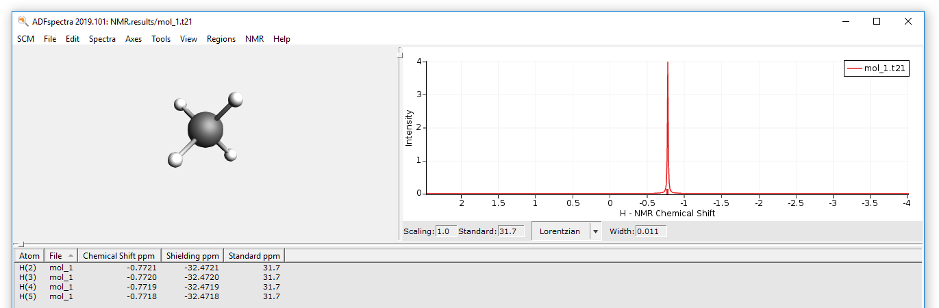
You can also open the result files for the individual calculations:

In ADFjobs click once on mol_1.t21 to select it

SCM → Spectra

Change the width of peaks to 0.01

Close ADFinput and ADFspectra

Conformers

The ADF-GUI does have some basic support for handling conformers. This includes the generation of conformers, the refinement of conformers using different theoretical methods, and the calculation of properties like spectra (UV/Vis, IR, NMR, and others). These spectra are the weighted spectra of the individual conformers, typically using a Boltzmann weighting.

The different conformers are stored in a .sdf file. The conformer handling is an example of handling multiple molecules.

The main steps to follow are:

• Generate and view the conformers (and thus the .sdf file that contains them)
• Refine the structures of the conformers, for example with ADF
• Calculate the spectrum of interest for selected conformers
• View the Boltzmann averaged spectrum

Each step will do something for all (or the selected) conformers. At the end of each step a new .sdf file is generated based on the results of the calculations. The original .sdf file is kept in the .results directory, with a timestamp, as a backup.

For this tutorial we will do this for a small example molecule: propanoic acid.

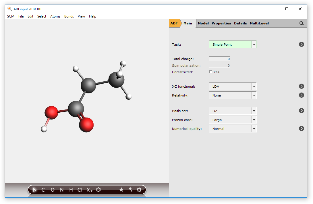
Step 3: Set up propanoic acid in ADFinput

Start ADFinput

Build propanoic acid (or search using the ADFinput search )

Step 4: Generate the conformers

Switch to the Conformers mode (use the orange ADF pull-down menu, used to switch methods)

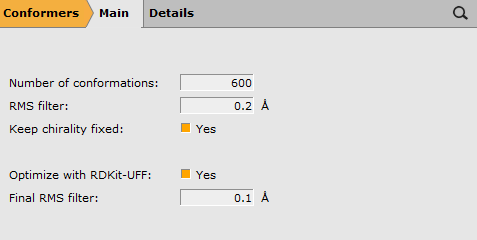
In this panel you set up how to generate the conformers (using RDKit).

The defaults should work fine: generate 600 random conformations, filter them with an RMS filter to avoid duplicate structures. Next optimize with RDKit-UFF so each conformation runs into some local minimum (conformer), and again filter with an RMS filter to avoid duplicate structures.

If you experience problems, or are curious, checking the Show log check box before generating the conformers will give some feedback during the conformer generation.

Note that the starting geometry does not matter, RDKit just looks at the connectivity and not at atom positions. The conformations are generated using distance-geometry conformation generator. For more info, see the RDKit web site.

Use File → Run (and save your molecule as ‘propanoicacid’)

Wait until the job is ready

In ADFjobs check that the propanoicacid job now contains a .sdf file (propanoicacid.sdf)

Use the SCM → Movie menu to view the conformers (it will automatically load the .sdf file)

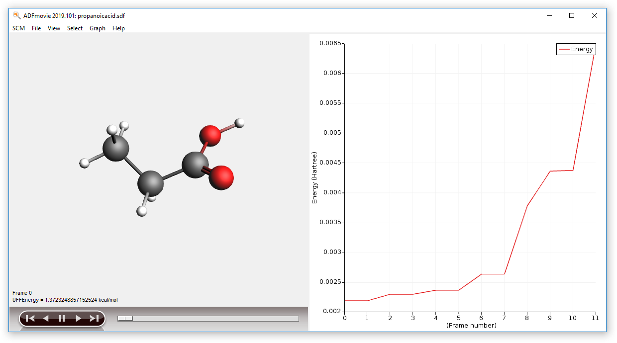
Using ADFmovie you can now examine the generated conformers. Note that the energy is the UFF energy as calculated by RDKit.

Step 5: Refine the conformer geometries with ADF

Next step is to improve the geometries of the conformers. If there are many conformers this may be expensive, so you may want to limit the conformers to be optimized to those with a certain energy range from the lowest conformer. Note that this energy range is a crude estimate by UFF. In the ADFmovie window you can see the energies of the conformers.

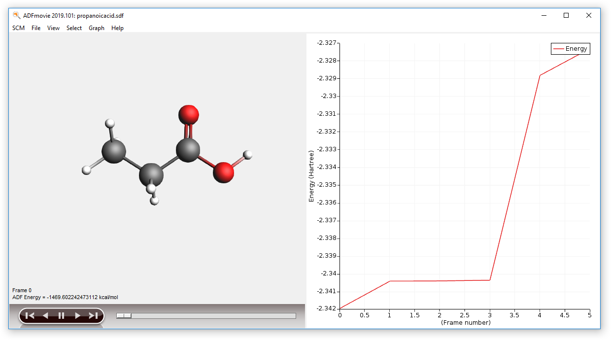
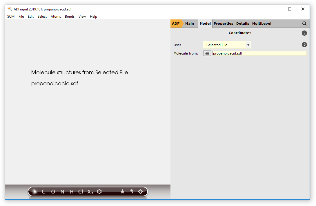
Close the ADFmovie window

In the ADFinput window switch to ADF mode and select the Geometry Optimization task

Switch to the Coordinates panel in the Model section

Use ‘Selected File’

Select the propanoicacid.sdf file in the ‘Molecule from’ field

Go to the ‘SDF Filter’ panel

Select all conformers with energy below 10 kcal/mol

Set the post-processing options: Sort, Remove duplicates between 0.1 Angstrom, and Align

Other options: move the mouse over them and check the balloons, the default values are correct

These settings in the Coordinates panel will run your job (whatever you specify in ADFinput to do, a geometry optimization right now) for all selected conformers (in the SDF filter panel): the conformers within 10 kcal/mol from the lowest conformer. In this case that is all conformers we have. If you have many conformers you may wish to restrict the energy range to reduce computation time.

The Use ‘Selected File’ option will create a job for the geometry/geometries in the selected file. In this example a .sdf file is used with multiple molecules, but you could also have selected any other file that the ADF-GUI knows and which contains a molecule (a .t21, .rkf, .xyz, …).

If you would not have adjusted the options in the Coordinates panel, ADFinput will note that an .sdf file is present when saving the job. It will ask you if you want to use it or not.

After the calculations have been done, a new .sdf file will be created, the conformers will be sorted (by energy), filtered to avoid duplicates, and aligned. Normally you would use a better basis set, but for the tutorial we stick to the DZ basis set (to get some results fast).

Run your setup (File → Run, click Save to save your set up)

Once the job is running, follow it with ADFmovie (in ADFjobs SCM → Movie)

in ADFmovie show the energy (Graph → Energy)

Wait until the calculations have finished (around 7 minutes on a recent desktop machine)

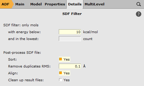
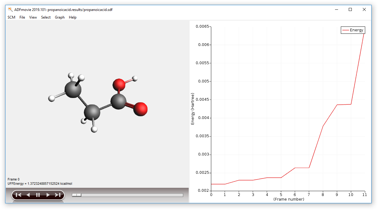
Close ADFmovie (showing the logfile)

Open ADFmovie (now it should show the new .sdf file, see title)

In the ADFjobs window open the details by clicking on the triangle

Locate the original .sdf file in the .results folder (with time stamp)

Click on it to select it

Open it in ADFmovie (SCM → Movie):

Show energy panel in ADFmovie window (Graph → Energy)

As you can see the conformer geometries and energies as optimized by ADF differ greatly from the UFF results:

In the ADFjobs window you could also select the results for individual conformers: select the result file of interest, and use the SCM menu (Output, Spectra, KF Brower, …) to examine it.

Step 6: Calculate the IR spectrum

To calculate the IR spectrum for all conformers (in the current .sdf file, with optimized ADF geometries), just set up an IR calculation in ADFinput as you would for a single molecule. And, just as for the geometry optimization in the previous step, the Coordinates panel will tell ADFinput to do this for all conformers.

As we also want to keep the current conformers (for example, to calculate different spectra), we will save the setup with a new name:

Close the ADFmovie windows

In ADFinput, use the Frequencies task (in the Main panel)

Select the Model → Coordinates panel

Make sure the “Use Selected File” is still selected

Make sure the Molecules are taken from the .sdf file from the previous step

File → Save As… and save the job with a new name (propanoicacid_IR)

File → Run

Wait until the calculations have finished (around 7 minutes on a recent desktop machine)

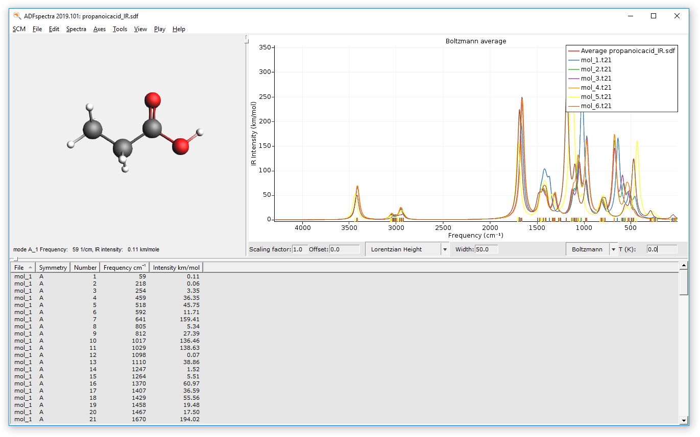
Step 7: Visualize the Boltzmann weighted IR spectrum

SCM → Spectra

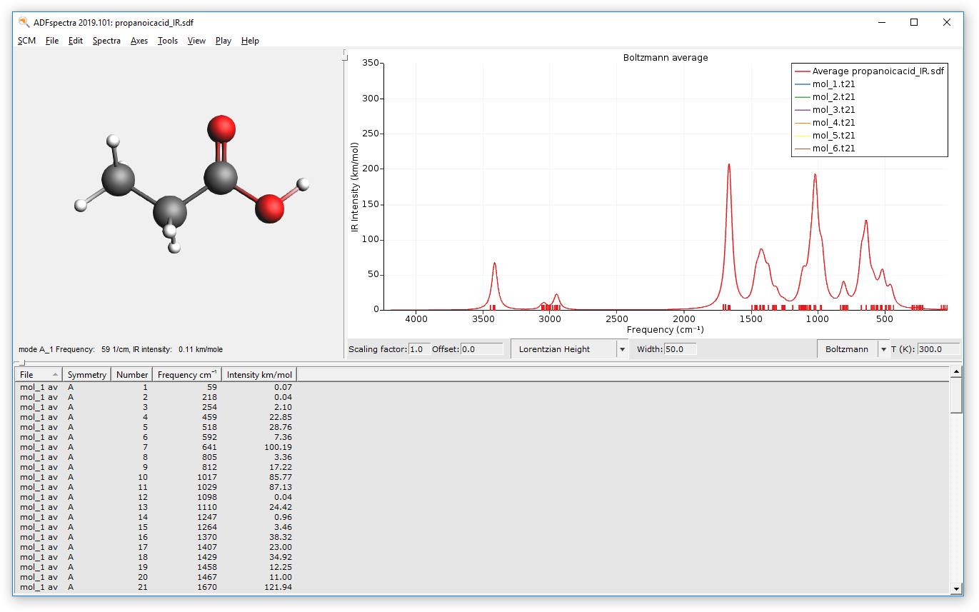
Change the temperature to 0 K

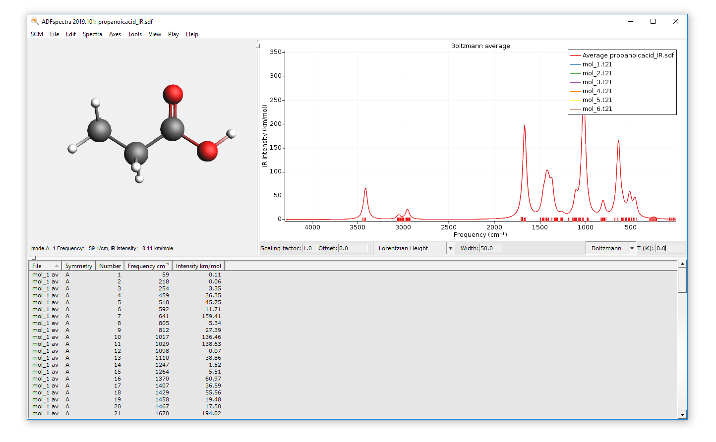
Obviously you can also select a high temperature, but the spectrum will be missing contributions from conformers that have been filtered away.

You can select what weights to use Boltzmann, Uniform or User defined:

Select “User Weights” from the weights pull down at the bottom

(the menu labeled “Boltzmann Averaged” at this moment. You may need to increase the size of your ADFspectra window for it to be visible.)

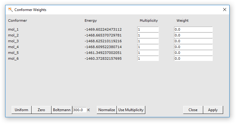
In the Conformer Weights window you can set the weight explicitly as you like for each conformer. You can use the buttons at the bottom to preset values. Move the mouse over the buttons and check the balloon help for more information. The multiplicity is the number of random RDKit conformations generated that ended up in the same conformer after optimization.

You can also see the IR spectra of the individual conformers all at the same time (in one graph):

Switch back to “Boltzmann Averaged”

Use the View → Average curve menu command to toggle between the average and all of the individual curves

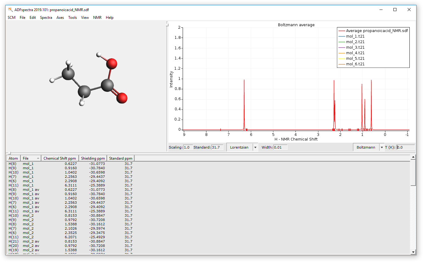
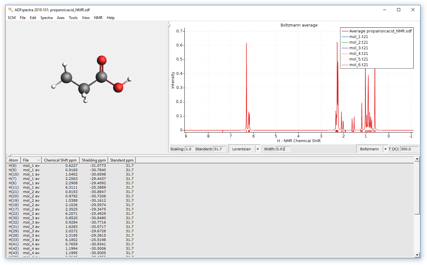
Step 8: H-NMR, UV/Vis

By now it should be evident how to set up calculations for all of the conformers. Two more examples: the H NMR spectrum and the UV/Vis spectrum.

Open the previous IR job in ADFinput

Change the Task to Single Point

Go to the NMR panel (in the Properties section)

Check the ‘Shielding for all H atoms’ option

Go to the Coordinates panel

Make sure the propanoicacid.sdf file is still used as source of conformers

File → Save As… and save it as propanoicacid_NMR

File → Run

Wait for the calculation to finish (around 1 minute)

SCM → Spectra

Change the width to 0.01

The final spectra (at 0K and at 300K) should like this:

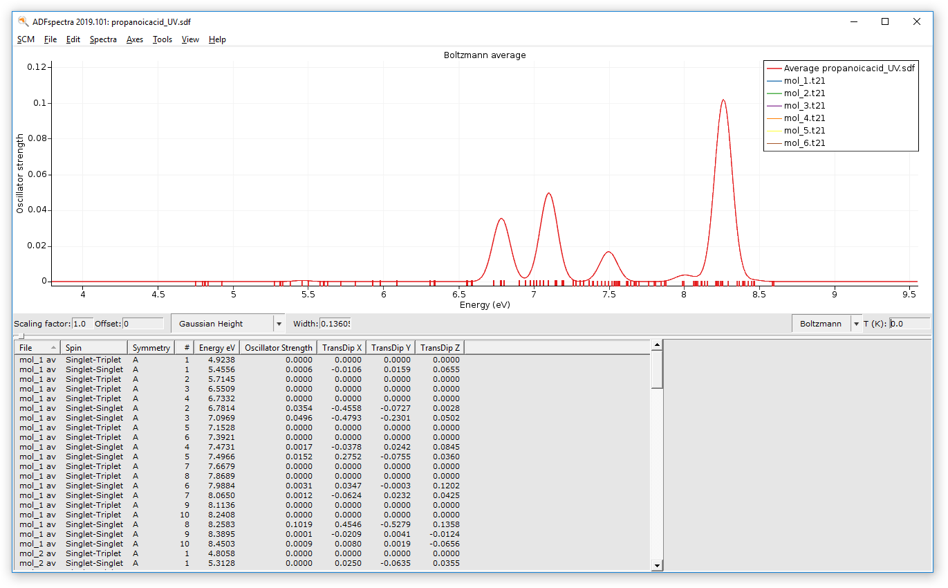
Calculate the UV/Vis spectrum (do not forget to turn off the calculation of the NMR spectrum)

Wait for the calculations to finish (around 3 minutes).

The final spectra (at 0K and at 300K) should like this:

Multiple Methods

You can also set up a series of calculations with different methods, and run them automatically one after each other. The geometries will automatically be passed from one job to the next.

As examples we first show how to set up a series like: DFTB optimization, ADF optimization and ADF UV/Vis spectrum for the optimized structure. We will then run this set up twice: once for the specified molecule, and once for a set of molecules.

Step 9: Set up a series of calculations

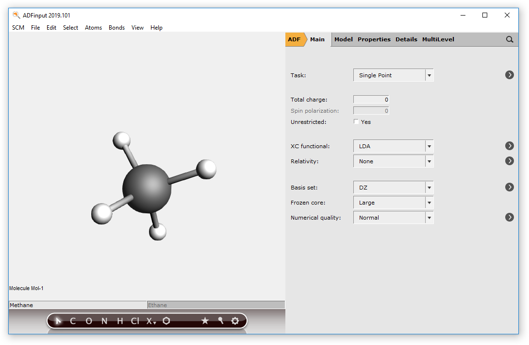
The first step in the series is a DFTB calculation on a molecule, we will use Acetone as an example:

Start ADFinput

Make (or find) an Acetone molecule

Switch to DFTB mode

Select the ‘Dresden’ parameter set

Save as ‘dftb’

Close ADFinput

The second step in the series is an ADF geometry optimization of the optimized structure from the first step:

Start ADFinput

Select the Geometry Optimization task

Switch to the Coordinates panel

Use Job Result

Molecule from dftb.adf

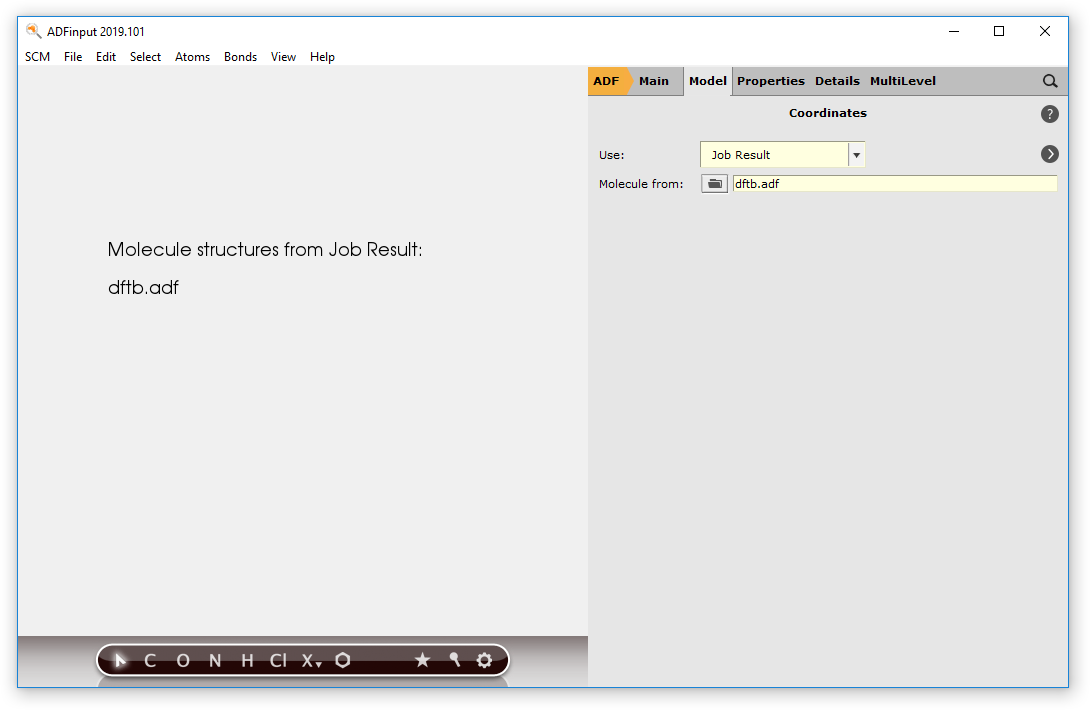
We now use the Job Result option in the Coordinates panel: this will make sure that the selected job is run first, and that the resulting geometry of that job will be used as input geometry for the current calculation.

Save as ‘adf-geo’

Close ADFinput

The third step in the series is an ADF UV/Vis calculation for the ADF-optimized structures:

Start ADFinput

Set up an UV/Vis calculation

Switch tot the Coordinates panel

Use Job Result

Molecule from adf-geo.adf

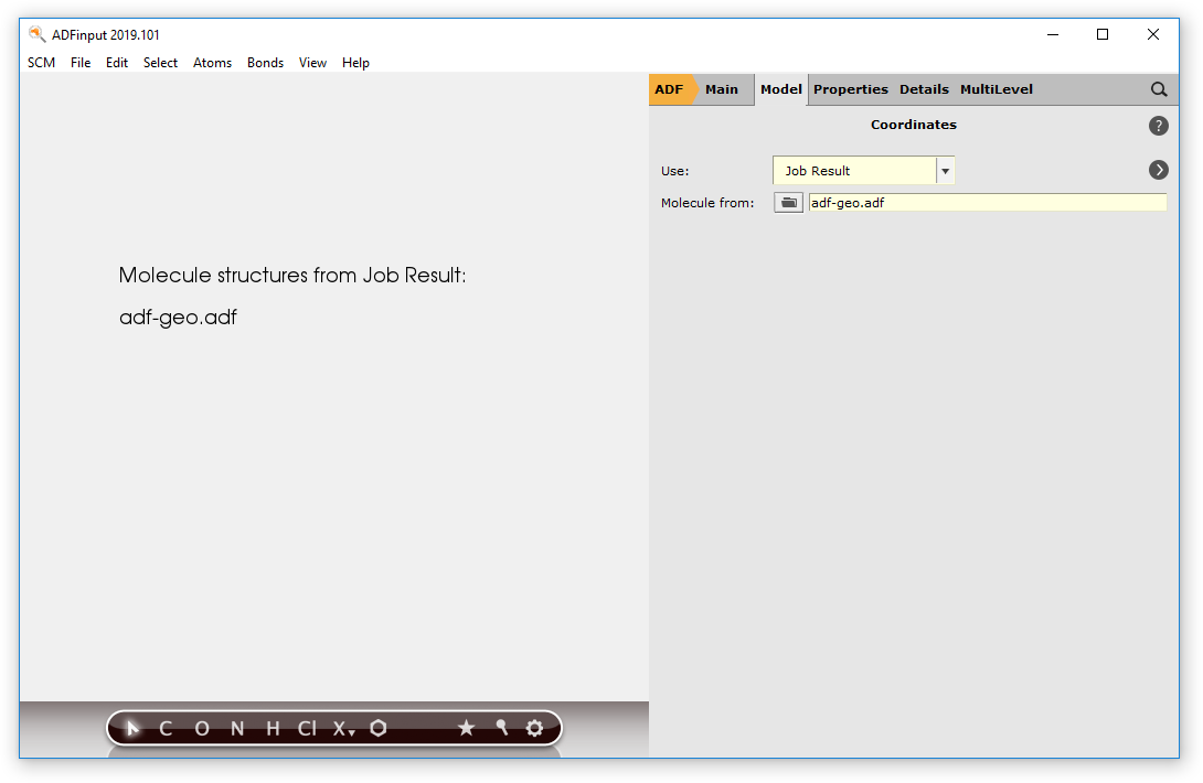
Save as ‘adf-uvvis’

Close ADFinput

Step 10: Run a series of calculations for a single molecule

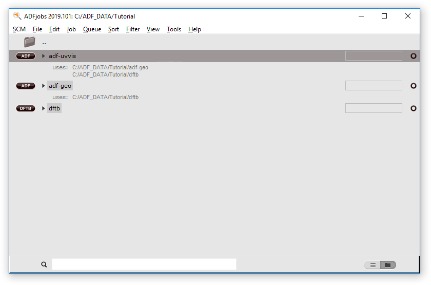
To run the just created series of calculation all we need to do is to start the final job (adf-uvvis). ADFjobs will detect that it uses results of other jobs, and start those jobs automatically:

Start ADFjobs (or make it active if it is still running)

Select the adf-uvvis job

In the ADFjobs window you can see on which jobs the selected job depends:

Run the job

In ADFjobs you should now see all the jobs in the job series running, one by one, in the proper order. If you wish you can examine the results of each job step as you would for normal independent jobs.

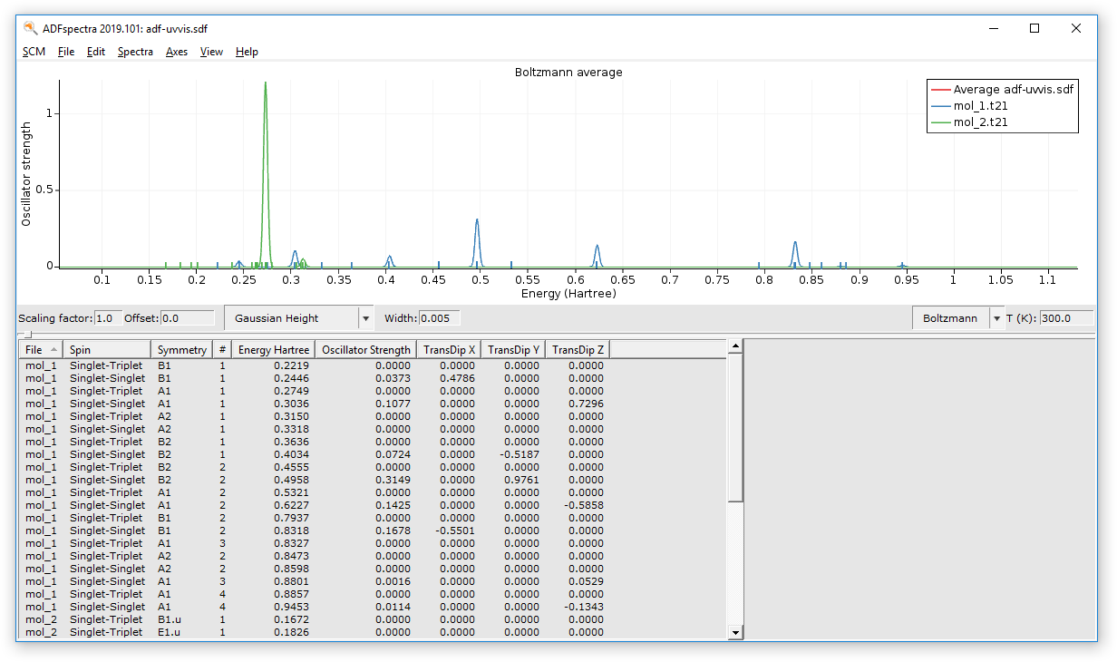
Lets now just check the final UV/Vis spectrum:

Select the adf-uvvis job in ADFjobs

SCM → Spectra

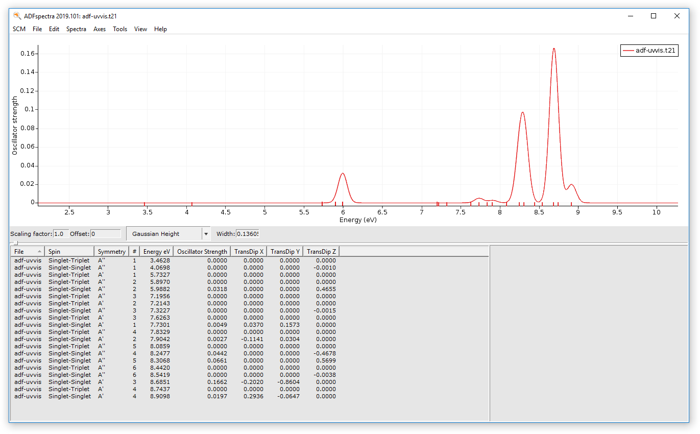
Remember that in the adf-uvvis job no molecule was specified, the geometry has been imported from the result of the adf-geo job. And that job in turn got the geometry from the dftb job.

Step 11: Create an SDF file, and Run a series of calculations for a set of molecules

The series of calculations in the previous steps can also be run with molecules from a .sdf file as input. Any SDF file can be used, for example the earlier sdf files from this tutorial.

In this case we will make a new SDF file just to show how to do that as well. First we make two .adf files, one for benzene and one for water:

Start ADFinput

Make benzene

Save as benzene.adf

File → New

Make water

Save as water.adf

Close ADFinput

Next we make an SDF file containing the two molecules we just made:

Go to ADFjobs

Select the benzene and water jobs you just made (use control click to select multiple items)

Tools → Add To SDF…

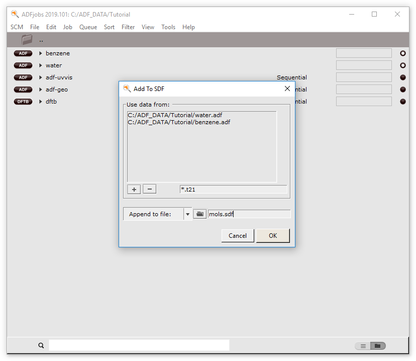
In the Append to file option select a name for the .sdf file to create: mols.sdf

Click OK

A new SDF file with the specified name will be created, containing the structures you selected. You can also add extra molecules to the .sdf file using the same method (just select an existing .sdf file instead of a new one). You can also include structures resulting from calculation results you have (.t21, .rkf files etc), or even from simple .xyz or .mol files and so on/

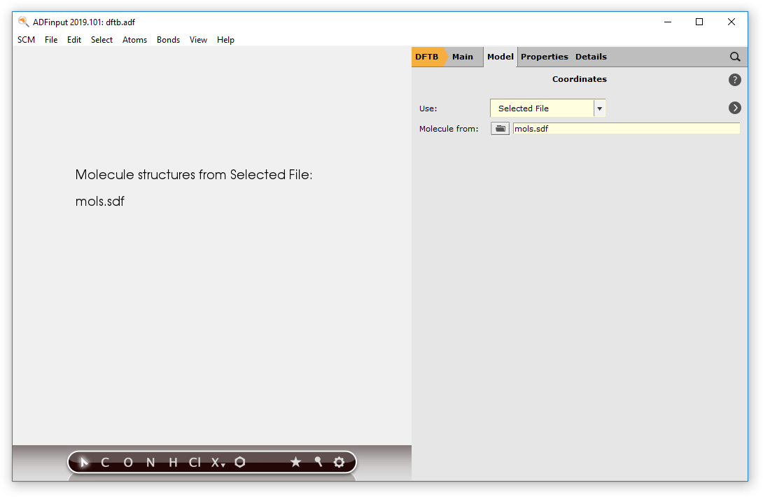
Next we want to run the series of jobs (DFTB - ADF geometry optimization - ADF UV/Vis) for all molecules in the mols.sdf file. In the first job of the series (DFTB) specify to use molecules from the .sdf file:

Open the dftb.adf file in ADFinput again (click No when asked to update coordinates)

Go to the coordinates panel

Use Selected File

Molecule From: select the mols.sdf file just created

File → Save

In ADFjobs select the last job in the series (adf-uvvis)

Job → Run

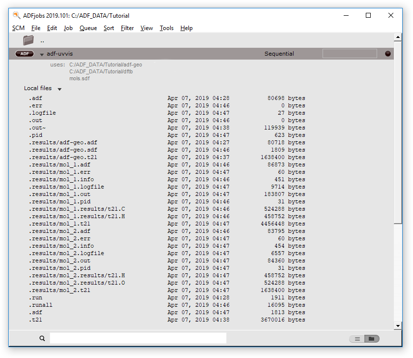
You should see all jobs running again in ADFjobs, but now multiple times. In the .results directories you will find the results for the individual jobs, and the final geometries are always collected in new .sdf files.

In ADFjobs show the details of the adf-uvvis job (click on the triangle)

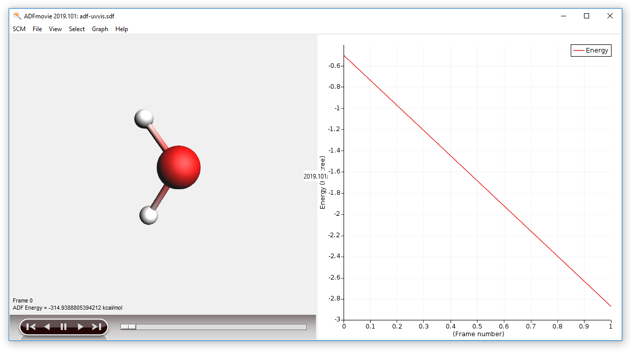
As before you can see the average or individual spectra via ADFspectra, or the geometries using ADFmovie:

SCM → Spectra (with the adf-uvvis job selected)

In the ADFspectra window: View → Average/All Curve

SCM → Movie (with the adf-uvvis job selected)