Periodic Energy Decomposition of the Tetrahydrofuran/Si(001) System
The creation of organic/inorganic interfaces is relevant to enhancing the range of applications of modern electronics. Understanding the driving forces that bind an organic molecule onto a metal surface is therefore highly important in this context. Naturally, such an understanding involves more than just simple interaction energies, i.e. \(E_{\mathrm{interaction}} =\) \(E_{\mathrm{molecule+surface}} – E_{\mathrm{surface}} – E_{\mathrm{molecule}}\). To this end, the well-established energy decomposition analysis (EDA) represents such a more detailed approach to bonding analysis. EDA has recently been extended to periodic systems. This periodic energy decomposition analysis (PEDA) approach is available in BAND, where it can be used to study cases like molecular adsorption on extended surfaces.
Based on a recent study
L. Pecher and R. Tonner Deriving bonding concepts for molecules, surfaces, and solids with energy decomposition analysis for extended systems, WIREs Comput Mol Sci., (2018).
this tutorial details the workflow for a periodic energy decomposition analysis on the example of a tetrahydrofuran (THF) molecule on a silicon slab model.
PEDA decomposes the interaction energy between molecular fragments into the well-defined energy terms for the Pauli repulsion, the electrostatic interaction, and the orbital relaxation. If PEDA is furthermore combined with so-called “natural orbitals for chemical valency” (PEDA-NOCV), the orbital relaxation can be split up further into components between NOCV pairs. Additional visualization of the respective NOCV deformation densities allows then to associate these components with e.g. the formation of σ- or π-type bonds.
These terms will be used in the following to describe the chemical nature of the interaction of THF with the silicon surface.
Model
We begin the Tutorial by loading the atomic model for the Si(001)-THF adsorption complex from a periodic xyz-file.
This structure was obtained by cuts along the [001] Miller plane in order to create a six-layer slab. The atoms at the bottom of this slab was then saturated by adding hydrogen atoms at the experimental Si-H bond length of Silane (1.48 Å). The unit cell was extended to form a 2x4 supercell model. This resulting slab model was then relaxed while keeping the bottom two Si-layers and the hydrogen atoms fixed. On the surface of the slab there are two exposed Si-atoms, which form a characteristic alternating buckled structure. A further analysis reveals that this buckling (or symmetry breaking) is the consequence of each of the exposed Si-atoms having an unpaired electron. In consequently, one of these unpaired electrons transfers to the neighboring Si-atom and forming a lone pair with the other unpaired electron there. The Si center where the lone pair is located becomes more nucleophile and gets pushed upwards (Siup) while its more electrophile neighbor (Sidown) moves slightly towards the slab.
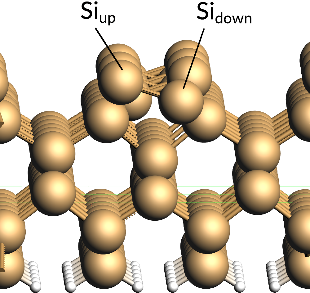
Due to the electrophile nature of Sidown the THF molecule was then added on top of this site with its O-atom oriented towards Sidown. Afterwards, the resulting adsorption complex was relaxed to yield the structure provided for this tutorial.
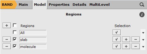
The periodic structure is loaded by opening the file THF_Si001_DativeBond.xyz with adfinput. As this structure file includes lattice vectors, this will automatically switch to the calculation options for BAND. Next, the regions of the adsorption complex need to be defined in order to analyze the interactions between them with PEDA.
- In the options tab of adfinputModel → RegionsRemove any existing regions by clicking on the “-” button on their leftSelect all Si-atoms and the H-atoms at the bottom of the slabClick on the “+” button and name the newly defined region e.g. slabUnselect and select all atoms of the THF moleculeClick on the “+” button and name the newly defined region e.g. molecule

Settings
Based on the regions defined above, PEDA will invoke three individual DFT calculations, one for each fragment and one for the whole adsorption complex, respectively.
Note
We calculate the fragments in their respective singlet states as we are targeting a donor-acceptor type bonding situation. In the case of multiple bonds or bonds which result in radical species upon dissociation it might me necessary to test different spin configuration (i.e. the configuration with the smallest absolute value of E_orb, see below)
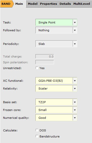
We specify the options for the DFT calculations as follows:
- In the options tab of adfinputClick on MainSelect XC functional: → GGA-D → PBE-D3(BJ)Relativistic: → ScalarBasis set: → TZ2PFrozen core: → SmallNumerical quality: → Good
PEDA itself can handle an arbitrary k-space grid, which is often necessary for cases like metallic surfaces. However, PEDA-NOCV is only implemented for a Gamma-only k-space grid. We set this option as follows:
- In the options tab of adfinputClick on Details → K-Space IntegrationSelect K-Space: → Gamma Only
Also any symmetry treatment needs to be disabled:
- In the options tab of adfinputClick on Details → SymmetryUntick Use Symmetry
We proceed by enabling the usage of fragments in ADF:
- In the options tab of adfinputClick on MultiLevel → FragmentsTick Use Fragments

Finally, PEDA-NOCV needs to be activated as follows:
- In the options tab of adfinputClick on Properties → PEDA-NOCVTick Perform PEDA-NOCV Analysis

After everything is set, save the ADF input with File → Save As… and start the calculation with File → Run.
Note
The individual input scripts which can be used from the commandline are available from the links listed below. Note, that PEDA.run depends on the results of the other two input scripts and needs therefore to be executed last.
PEDA Terms
After completing the calculation we can examine the results as follows:
- SCM → Output to switch to ADFoutputProperties → PEDA Energy Terms
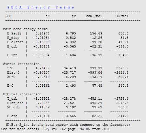
Here E_int denotes the total interaction energy between the two fragments, i.e. between the Si(001) slab and THF.
PEDA subdivides this interaction into components corresponding to the Pauli repulsion E_Pauli as well as dispersion E_disp, electrostatic E_elstat, and orbital interactions E_orb, which are found in almost perfect agreement with the original study:
| PEDA terms | Present [kJ/mol] | Pecher & Tonner [kJ/mol] |
|---|---|---|
| E_pauli | 655.6 | 656 |
| E_disp | -51.3 | -51 |
| E_elstat | -415.1 | -417 |
| E_orb | -344 | -344 |
| E_int | -154.8 | -156 |
Due to the elecrophile character of Sidown we can expect a dative bond between the THF O-atom and this site.
Indeed, the E_orb and E_elstat interactions are found both rather high with values of several hundred kJ/mol and the latter slightly dominating (54-55%), which are typical features of dative bonds.
NOCV Orbitals
To analyze the dative bond between Sidown and THF further, we proceed by examining the natural orbital for chemical valence (NOCV).
- In ADFouput SCM → View to switch to ADFviewFields → Grid → Medium (or Fine)Add → Isosurface: With Phase
This creates an empty field to plot which can be adjusted in the bar at the bottom:

- In the field options barChange the isosurface value from 0.03 to 0.0025Select Field … → NOCV Def Densities…
Hint
In the field options bar, Isosurface: With Phase → Show Details provides access to further plotting options such as transparency
This will open a window containing the different NOCV orbital pairs sorted according to their contribution to the deformation density:
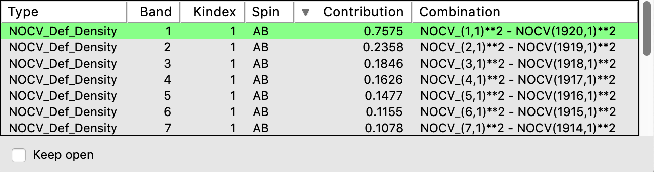
- In the window Select NOCV Deformation DensityDouble-click on the first entry (largest contribution),
NOCV_(1,1)**2 - NOCV_(1920,1)**2
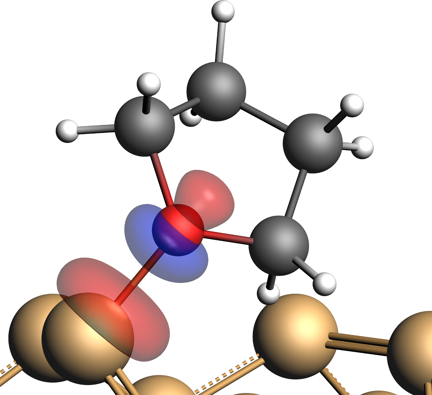
This will show a plot of the NOCV pair contribution to the deformation density:

This plot is to be interpreted as follows: Red lobes show an electron depletion due to the fragment interactions while blue lobes represent an increased electron density. The above plot shows that electrons are removed from the surroundings of the O-center (and to a lesser extend from Sidown) and accumulated in between these two atoms, which is a clear indication for the formation of a bond. We can examine this bond further by looking at the two NOCV orbitals that form the NOCV pair.
- Add → Isosurface: With Phase to add another field options barIn new field options bar: Change the isosurface value from 0.03 to 0.0075Click on Select Field … → NOCV Orbitals…In the selection list: double-click on the first NOCV orbital (most negative contribution)Repeat these steps for the last NOCV orbital (with the largest contribution)
Hint
By ticking or unticking the leftmost box in each field option bar you can hide or show the individual plots
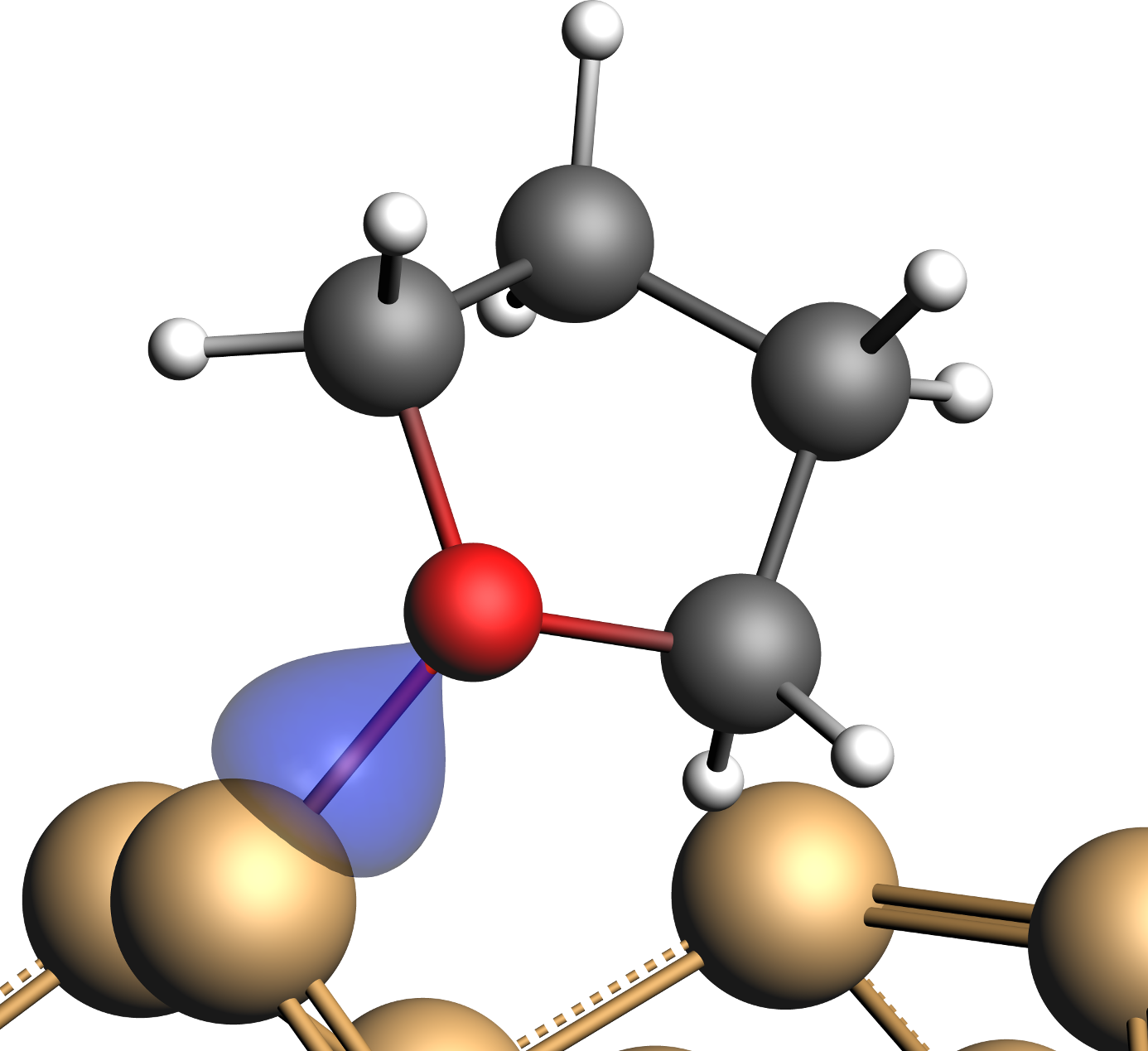
For a given pairs of NOCVs the one with the lower index corresponds to the electron donor orbital and the orbital with the higher index is its electron accepting partner. The NOCV on the left thus derives from the lone pair at the O-center, while the orbital on the right side originates from unoccupied orbitals of the Sidown atom.
Note
NOCV orbitals emerge as the result of several orbital transformations and their interpretation might not always be easily possible.