Parallel scalability of Elastic Tensor calculations
In this tutorial we will use the DFTB engine to calculate the elastic properties of a zeolite. Using this system as an example, we want to explore the parallel scalability of the calculation the of elastic tensor elements
of a crystalline material. Here \(V_{0}\) denotes the volume of the unit cell, \(\epsilon_{\alpha}\) and \(\epsilon_{\beta}\) the strain elements (in Voigt notation), while \(E\) stands for the systems total energy.
Technically the first step in the calculation of an elastic tensor is a very tight optimization of both the nuclear and lattice degrees of freedom. Once the equilibrium configuration is found, the lattice is artificially strained and the nuclear degrees of freedom optimized again. This last step has to be repeated 84 times with different lattice strains in order to obtain the 21 unique elements of the 6x6 elastic tensor using a two-sided numerical differentiation.
This makes for an interesting and yet realistic example application to study the parallel scalability of the AMS driver and its engines:
- The initial geometry optimization (including the lattice degrees of freedom) is inherently serial at the driver level: every step can only be started after the previous step has finished. Any parallel speedup can only result from the in-engine parallelization, i.e. each individual step taking less time.
- The subsequent 84 optimizations with the strained lattices can be executed in parallel, as they are completely independent from each other. However, some of these optimization may take more steps than others, creating a potential load balancing problem: after all, the calculation of the elastic tensor is only complete when the last optimization finishes!
This situation poses some interesting questions:
- How scalable is the initial optimization of the lattice degrees of freedom?
- How scalable are the subsequent parallel optimizations of the strained systems?
- What is the best parallelization strategy for the second part? Should we attempt to run as many of these 84 optimization as possible in parallel, or should we (in view of the mentioned load-balancing problem) dedicate more of our computational resources to each individual optimization, trying to finish it quickly?
Setting up the job
The specific zeolite we are going to use for this tutorial is an all silicon version of the large pored ITT framework. The original ITT structure was obtained from an online database, and its Ge atoms exchanged for Si-atoms. Let us first import the structure into ADFinput.
- 1. Start ADFjobs2. Open ADFinput by clicking SCM → New Input3. In the menu bar, click File → Import Coordinates…4. Download and select file
ITT.xyz
Next we should set up the engine we want to use for this calculation: We are going to use DFTB with the matsci-0-3 parameterization and the D2 dispersion correction.
- 1. Switch to DFTB:
 →
→  2. Select Parameter Directory: → DFTB.org/matsci-0-33. Select Dispersion: → D2

We now set up the initial optimization of both the nuclear and lattice degrees of freedom. It is very important to choose rather tight convergence criteria for this initial optimization. Otherwise the uncertainty in the final energy of the initial optimization might be of the same order of magnitude as the energy differences upon straining the system, resulting in a noisy elastic tensor.
Hint
The convergence criteria used for the initial optimization in this tutorial match those used for the calculation of the elastic tensor, see the manual entry for further information. This should be considered the minimal strictness that gives reliable results. However, for production calculations of elastic tensors we recommend to choose a bit tighter convergence criteria.
- 1. In the panel bar, select Details → Geometry Optimization2. Check the Optimize lattice checkbox3. In Gradient convergence enter
1.0E-4Hartree/A4. In Stress energy per atom enter5.0E-5Hartree

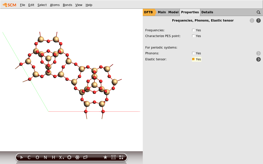
Finally we need to enable the calculation of the elastic tensor.
- 1. In the panel bar, select Properties → Frequencies, Phonons, Elastic tensor2. Check the Elastic tensor checkbox
This concludes the setup of the job.
Measuring parallel scalability
We now want to investigate the parallel scalability of the job we have just set up. The parallelization in AMS, both on the driver level and inside the engine, works completely automatically. While it is possible to manually influence the parallelization strategy, see the respective page in the AMS driver manual, it is usually best to just give AMS an appropriate amount of computational resources and otherwise rely on the automatic parallelization setup. We will therefore just run the exact same job multiple times, giving it more or less computational resources, and will simply record the total run-time of the job to judge the efficiency of the parallelization.
How exactly we continue at this point depends on which machine we want to run this scalability study on. It is possible to follow this tutorial by running all jobs sequentially on your local machine, using a varying number of CPU cores. For users that have access to a compute cluster it is however recommended to submit the jobs to the cluster using ADFjobs’ remote queues. Not only will this be faster, but it will also be more instructive since your local machine likely does not have enough CPU cores to reach the limit of parallel scalability for this jobs, i.e. the point where adding more computational resources no longer reduces the job’s run time. If you have access to a compute cluster, but have not yet set up remote queues for it, we recommend to do so now. You can find instructions on how to set up remote queues in the installation guide and the ADFjobs manual.
No matter where we actually run these jobs, for every parallel setup we want to test (e.g. 1 core, 2 cores and 4 cores), we will save a copy of the job under a unique name and run it:
- 1. In the menu bar of ADFinput, click File → Save As…2. Select a unique name representing the parallel setup you want to test in this job, e.g.
ITT_4coresfor the job that you want to run on 4 CPU cores.3. In ADFjobs: type the number of cores you want for that job into the field to the right of the job’s name.4. Repeat step 1. to 3. for all parallel setups you want to test.5. Optional: Assign the job to one of your remote queues by clicking in the menu bar: Queue → [Name of your queue]6. Submit the job to the queue by clicking Job → Run in the menu bar.

For the purpose of making this tutorial we ran the job on a cluster of dual socket machines with two 16 core Intel Xeon Gold 6130 processors each. We have therefore set up jobs measuring the scalability within a single node (using 1, 2, 4, 8, 16 and all 32 cores of the machine) as well as multi-node jobs using 2, 3 and 4 of the cluster’s nodes. Four nodes with 32 cores each is likely too much resources for an efficient parallelization of this relatively small system with the rather fast DFTB engine. This is on purpose, as we would like to show that parallel scaling over a wide range of setups, up to the point where the job is just over-parallelized and does not scale anymore.
Once the jobs are running, we can visualize the progress of the initial geometry optimization in ADFmovie.
- 1. Select one of the calculations in ADFjobs2. Open it in ADFmovie by clicking SCM → Movie
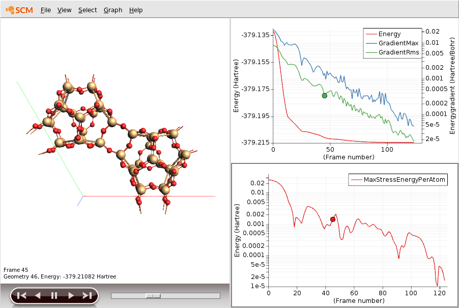
ADFmovie only shows the progress of the initial optimization. Once the job has finished this part and is busy with the elastic tensor calculation we can monitor its progress by looking at the logfile.
- 1. Select one of the calculations in ADFjobs2. Open its logfile by clicking SCM → Logfile
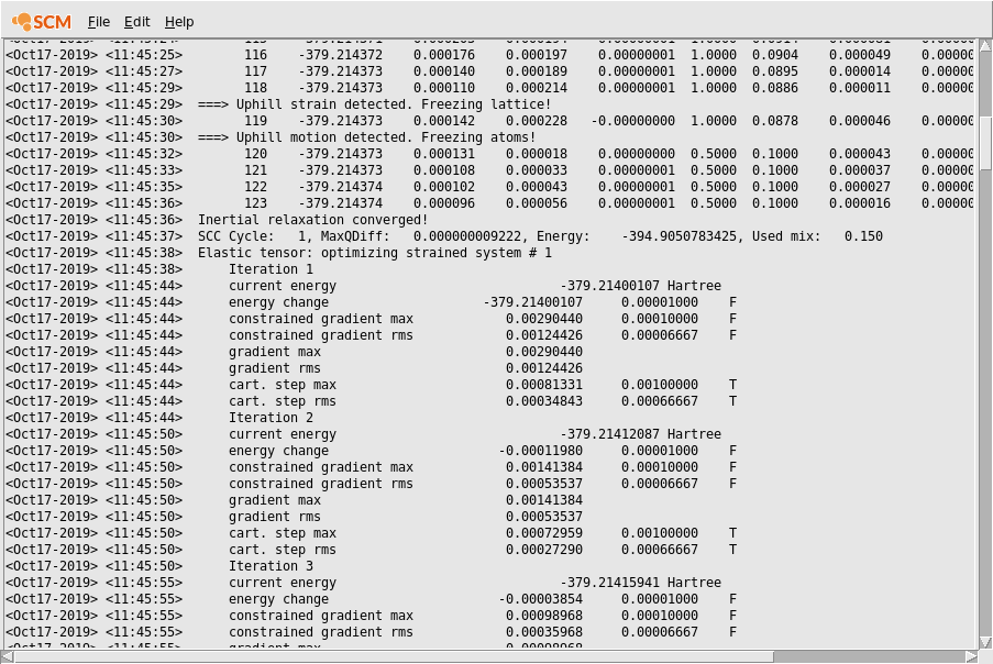
Scrolling up we can see both the output from the initial optimization of both nuclear and lattice degrees of freedom, as well as the subsequent optimizations of the strained systems. We will later use the times printed in the logfile to measure both the scalability of the initial geometry optimization and the elastic tensor calculation.
If you scroll through the logfile you will see the lines containing Elastic tensor: optimizing strained system followed by a number. These are the 84 individual geometry optimization of the strained systems we mentioned in the introduction of this tutorial. Note that unless you are running the job completely serially you will not see all of these 84 optimizations in the logfile: As the individual optimizations are completely independent from each other, they will automatically be parallelized at the AMS driver level. Technically all available CPU cores are split up into groups. Cores in one group work together on a single optimization, and after finishing it will move on to the next independent optimization that has not yet been picked up by another group. The logfile you see is written by one of these groups (the one that contains the first CPU core on the first node), so you only see the messages relating to the optimizations that have actually been picked up by that specific group. The parallel part only ends when all 84 optimization have been picked up by a group, and the last group still working has finished its last optimization. At this point all groups merge again, the results are collected, and the elastic tensor calculated.
The big question at this point is how many groups should be created? Unfortunately this question is fairly hard to answer. There are many competing effect that should be taken into account here.
- How big is the system and how many cores can be utilized efficiently by the engine for this size of system? We do no want to create groups that are so big that the parallel scalability inside of the group suffers.
- How much memory will each group need? Often the amount of memory needed is determined by the system size alone. We do not want do calculate so many systems in parallel that we run out of memory.
- The 84 individual optimization of the strained systems will not all take the same number of steps. Some will finish within a few steps, while others might take 40 steps to converge. This means we probably do not want to create too many and hence slow groups: If we had 84 groups, 83 of them would at the end just wait for the one group whose optimization takes the most number of steps.
These are not the only considerations going into the decision. We likely also want to prefer creating equally sized groups, prefer group sizes that are a power of 2 (which is best for some of the distributed memory linear algebra operations), and in order to reduce inter-node communication also avoid groups that span multiple nodes. In summary: it’s complicated!
Luckily the end-users is not expected to make these decisions. It is possible to manually set the number of groups, see respective page in the AMS driver manual, but generally we recommend letting the AMS driver handle the parallelization automatically. It is however possible (and for the purpose of this tutorial maybe instructive) to take a peek under the hood and get some additional info from AMS about the parallelization decisions it makes. This can be done by typing Info MultiLevelIteratorModule into the Log field on the Details → Expert AMS panel in ADFinput. This produces a fair amount of output, which is mostly intended for developers. But here is part we care about for the job that ran on 2 of the 32 core nodes:
Log MultiLevelIteratorModule:Info --- entered AutomaticNumberOfGroups
Log MultiLevelIteratorModule:Info --- nTasks = 84
Log MultiLevelIteratorModule:Info --- costRatio = 4.000000
Log MultiLevelIteratorModule:Info --- possibleNumGroups = 1 2 4 8 16 32 64
Log MultiLevelIteratorModule:Info --- nGroups = 1
Log MultiLevelIteratorModule:Info --- groups too large: badness + 6.111111
Log MultiLevelIteratorModule:Info --- overall badness = 6.111111
Log MultiLevelIteratorModule:Info --- nGroups = 2
Log MultiLevelIteratorModule:Info --- groups too large: badness + 2.555556
Log MultiLevelIteratorModule:Info --- overall badness = 2.555556
Log MultiLevelIteratorModule:Info --- nGroups = 4
Log MultiLevelIteratorModule:Info --- groups too large: badness + 0.777778
Log MultiLevelIteratorModule:Info --- overall badness = 0.777778
Log MultiLevelIteratorModule:Info --- nGroups = 8
Log MultiLevelIteratorModule:Info --- overall badness = 0.000000
Log MultiLevelIteratorModule:Info --- nGroups = 16
Log MultiLevelIteratorModule:Info --- overall badness = 0.000000
Log MultiLevelIteratorModule:Info --- nGroups = 32
Log MultiLevelIteratorModule:Info --- no load balance averaging: badness + 0.523810
Log MultiLevelIteratorModule:Info --- overall badness = 0.523810
Log MultiLevelIteratorModule:Info --- nGroups = 64
Log MultiLevelIteratorModule:Info --- no load balance averaging: badness + 2.047619
Log MultiLevelIteratorModule:Info --- overall badness = 2.047619
Log MultiLevelIteratorModule:Info --- selected nGroups = 16
What does this mean? There were 84 tasks to be done and the estimate was that some of them might be 4x more expensive than others, due to the varying number of steps in the geometry optimization. The AMS driver considered splitting the 64 available CPU cores into 1, 2, 4, 8, 16, 32 and 64 groups. 1, 2 and 4 groups were considered bad because it would lead to groups that are too large to have an efficient internal parallelization, given the fixed size of the system. Making 32 groups of two cores each or even creating 64 core “groups” of just one core were both considered inefficient as each group would only have a few optimization to do: too few to average out that some of them are more expensive than others. Ultimately the AMS driver decided to make 16 groups of 4 cores each. This was considered a good compromise between having not too large groups but still having enough tasks per group.
This being said, let us now look at the actual numbers for the scalability of our job:
| nCores | Initial GO | Speedup | Elastic tensor | Speedup | Total time | Speedup |
|---|---|---|---|---|---|---|
| 1 | 1517s | 1.0x | 13500s | 1.0x | 15017s | 1.0x |
| 2 | 948s | 1.6x | 6360s | 2.1x | 7309s | 2.1x |
| 4 | 528s | 2.9x | 3538s | 3.8x | 4066s | 3.7x |
| 8 | 340s | 4.5x | 1977s | 6.8x | 2317s | 6.5x |
| 16 | 222s | 6.8x | 898s | 15.0x | 1120s | 13.4x |
| 32 | 211s | 7.2x | 621s | 21.7x | 832s | 18.0x |
| 2x32 | 228s | 6.6x | 429s | 31.5x | 657s | 22.9x |
| 3x32 | 250s | 6.1x | 336s | 40.2x | 586s | 25.6x |
| 4x32 | 294s | 5.2x | 288s | 46.9x | 582s | 25.8x |
- As expected, the inherently serial initial optimization does not scale well. The system is just too small for the DFTB engine to scale well beyond a few CPU cores. The maximum speedup is observed when using the entire node with all its 32 cores. However, this is only marginally faster than using only 16 cores. Using more than 1 node is counter productive for this kind of system and makes the initial geometry optimization slower. Luckily the inherently serial initial optimization only represents a small part of the overall run-time.
- The much more expensive elastic tensor calculation also scales much better.
- The more parallel the job runs, the larger is the relative amount of time spent in the initial geometry optimization. For the most parallel setup with 4x32 cores we actually spent more time in the initial optimization than in the calculation of the elastic tensor.
Knowing what we know now, it is fair to say that our job scales up to roughly 32 CPU cores. Beyond that it’s hard to justify the expense of computational resources for the small additional speedups. Your runtimes may be different depending on the machine that you ran the test on, but the general trends should be the same everywhere.
So what is the take-home message of this tutorial?
- Parallelization in AMS, both at the driver level and inside the engines, happens completely automatically. The user just needs to give AMS an appropriate amount of computational resources and AMS will decide how to best make use of them.
- If the job contains an inherently sequential part (e.g. an initial geometry optimization as in this example) the overall scalability of the job may be limited by this sequential part, see Amdahl’s law on Wikipedia.
- Bigger systems and more expensive engines generally also scale better. We advise users to run some test on how well the engines that they use scale for a particular system size, and especially what is the maximum amount of CPU cores that is still efficiently utilized for a given system size. These can be very rough rules of thumb, e.g. that for DFTB one should have less than 10 atoms per used CPU core, but it is important to have this rough understanding.
This concludes the tutorial on parallel scalability.
Looking at the results
We got so carried away by the topic of parallel scalability that we never actually looked at the results of our calculation … Let us do this now!
- 1. Select one of the finished calculations in ADFjobs2. Open its text output by clicking SCM → Output3. Type
Elastic moduliin the search bar at the bottom4. Scroll up a little to also see the elastic tensor

As you can see the elastic moduli of our zeolite are roughly in the range as those of other minerals, see for example the page on isotropic elastic properties of minerals on the PetroWiki.org website.