Adsorption of CO₂ on a MgO Surface

Contents

This tutorial will lead you through the workflow of how to create a surface for a quantum chemical calculation and how to study adsorption of a molecule on this surface. A single crystal (of average macroscopic size) can have several cm² of surface area and a typical length scale treated with quantum chemistry would be around 10 Ų which is a factor of 10¹⁵ smaller than the average real crystal facet. The following figure shows a crystal and a so-called slab representing a surface

Fig. 7 A crystal and its digital twin fit for a QM or MM calculation.

However, we can use periodic boundary conditions to mimic a vast surface and as ionic crystal such as MgO are very regular this is easily possible. Periodic boundary conditions for a surface mean that they are replicas in two dimensions and in the third one there is a limited thickness and “vacuum” below and above – we call this a slab. The Figure below shows a unit cell of a slab of MgO which is four layers thick and an expansion of two cells in each direction of the unit cell.

Fig. 8 A slab cell and it’s expansion.

The Contents

If you are familiar with continuum methods you may ask yourself why indeed we don’t build a real size digital twin of crystal and use a finite element solver to calculate what is happening on the surface if someone exposes it to CO₂ gas. The answer is we want study electronic properties and adsorption energies of an individual CO₂ molecule and its chemisorption. This can only be captured by an electronic method and to some extent by an atomistic method. We will use BAND and thus, will need to build a slab. The ADF GUI has a tool to cleave along planes within a crystal, but which ones do we choose?

Cleave the right plane

In a real crystal we can recognize faces and as MgO is cubic face centered (such as NaCl) we would expect some cubic crystallites. When a crystal grows certain faces can grow faster and some slower – the latter are the larger ones and offer more surface to e.g. catalytic activities. Stable surfaces of ionic crystals have a dipole moment of zero perpendicular to the surface. One can also calculate the surface energy, \(E_{SE}\), using:

\[\Delta E_{SE} = \frac{E_{slab}- nE_{bulk}}{2A}\]

Where \(E_{slab}\) is the relaxed energy of the cleaved system and \(E_{bulk}\) the energy of the same atoms when they are embedded in a crystal bulk. \(2A\) is the total surface area, i.e. both sides of the slab. This is a way to test several possible surfaces for stability. For any stable surface this energy must be positive. If this energy was negative the atoms would dissociate into their surroundings.

Also, there are only seven lattice systems one has to consider: cubic, hexagonal, tetragonal, rhombohedral, orthorhombic, monoclinic and triclinic. A good idea is to do a literature search to see if the surfaces have been studied theoretically or experimentally and whether certain surfaces are described as stable or catalytic active. For MgO the [100] surface is most stable. Our next move will be to find out what thickness of the surface is needed.

The thickness of the slab

Ideally, the thickness of the slab should not influence the bulk energy of MgO. We will create slabs of different thickness and calculate the bulk energy, the surface energy and decide on the thickness the slab should have. Start with switching to DFTB:

In ADFInput

1. Switch from to

2. Use the Search Tool ( ) to find MgO

3. Select the crystal one

Go to Edit → Crystal → Primitive to Conventional Cell

Click on the Slice tool ( )

In the dialogue window

1. choose 1 0 0 as Miller indices

2. and number of layers 1

3. Click Generate Slab

For clarity remove the Bonds:

1. Bonds → Remove Bonds in the menu bar

2. Visualize the Unit Cell View → Periodic → Show Unit Cell

You will see

As you sliced from the conventional cell a slicer layer comprises two MgO layers with four formula units of MgO.

Tip

You can use the Periodic display tool ( ) to see the next nearest neighbors:

We now want to calculate the binding energies:

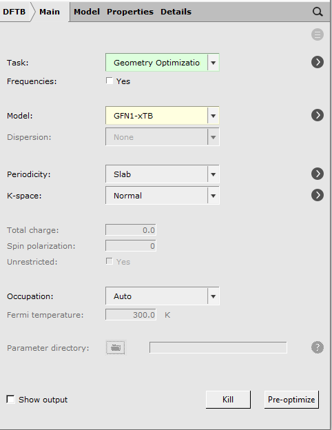
Choose Panel bar → Main

and change the calculation setup (Task and Model) according to the following picture

Note

As we want to later adsorb CO₂ onto MgO slabs it makes the most sense to adsorb it onto relaxed slabs. This is especially important for oxides. The issue is that simply bulk-truncating the bottom layer creates electronic states that can interact with whatever you put on the top layer. If you relax the whole slab, the occupied orbitals/bands will be lower in energy (more stable), meaning that they will have less interaction with the CO₂ you introduce at the top end of the slab. This means, DFTB will not transfer electrons from the bottom of the slab to the top, as the bottom-layer electrons are stable where they are. This may not be an issue for MgO, but for some other metal oxides, and for more redox-active adsorbates.

We also want to relax the experimental lattice parameters to get some adequate ones for the DFTB model we have chosen:

Choose Panel bar → Details → Geometry Optimization

and check Optimize Lattice

When the calculation has finished, open the “Output” using the SCM dropdown menu.

from select Output

Search for Total Energy and take a note of the second entry you’ll find.

use the one in eV

You will find

We will report the Final Bond Energy, i.e. -1195.57065033 eV.

Repeat this calculation for up to 9 layers and create a table. Remind yourself that each slicer layer is a double layer and comprises of four formula units, i.e. four Mg²⁺ and four O^2- atoms.

No. of MgO units/ slab	Total Energy [eV]
4	-596.3006119
8	-1195.57065
12	-1795.658628
16	-2396.16483
20	-2996.879832
24	-3597.675307
28	-4198.484686
32	-4799.259504
36	-5400.065737

If you remind yourself about the surface energy

\[\Delta E_{SE} = \frac{E_{slab}- nE_{bulk}}{2A}\]

We recommend not to compute this number directly since \(E_{slab}\) and \(E_{bulk}\) are sensitive to the k-point sampling and they have different periodicities as you would calculate \(E_{slab}\) 2D and \(E_{bulk}\) 3D, respectively. Hence, it will be difficult to make this consistent. Let us rearrange the equation:

\[E_{slab} = nE_{bulk} + \Delta E_{SE} \times 2A\]

Thus, plotting \(E_{slab}\) vs n should give a straight line where the intercept gives the surface energy (times the area, 2A) and the slope gives the “effective” bulk energy. This is the best way of calculating a surface energy. If you use the data from the table above and plot them with a program of your choice and generate a trendline you can get the slope and the intercept.

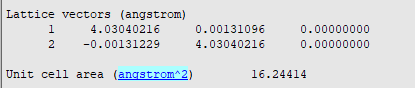
Thus, the bulk energy is -150.14 eV and \(\Delta E_{SE} x 2A = 5.4 eV\). You can find the value for A in your output file (use the last entry)

Thus, \(\Delta E_{SE} = 5.4 eV/2 x 16.24414 Å2 = 0.33 eV/Å2\). If we calculate \(\Delta E_{slab} = (E_{slab}^{m+1} - E_{slab}^{m/4}\) and plot this vs the number of double layers, we should obtain a function that converges towards the effective bulk energy.

No of double layers	Total Energy [eV]	ΔE_slab [eV]
1	-596.3006119
2	-1195.57065	-149.8175096
3	-1795.658628	-150.0219944
4	-2396.16483	-150.1265507
5	-2996.879832	-150.1787504
6	-3597.675307	-150.1988687
7	-4198.484686	-150.2023447
8	-4799.259504	-150.1937046
9	-5400.065737	-150.2015581

We can see from 12 layers onwards the binding energy is changing less and less, so it would be good to work with at least 12 layers. However, bear in mind that electronic calculations are expensive and an adsorption study will need a wider surface area, as we will discuss shortly. Thus, now it is time to rethink your methods and make sure you have access to a HPC or you decide to use a forcefield method. We will work with four layers to speed up the calculation time for this tutorial.

What could possibly go wrong?

Admittedly, MgO offers with [100] a well-behaved surface. With other surfaces you have to take care with how you cleave the bulk to not end up with a dipole moment:

Fig. 9 Some Ionic surfaces by P.W. Tasker .

Surfaces may have defects or are doped with other ions. In this case you cleave the surface and use the ADF GUI tools to remove or add atoms to build these defects. Be aware that everything you do to one surface is replicated due to periodic boundary conditions. You may want to use large enough supercells so that defects are better spaced out.

When you cleave surfaces like SiO2 or Si or Ge, the top layer has atom that lose their coordination because due to cleaving some neighboring atoms are removed. These surfaces have the ability to “self-heal” or reconstruct. In this case you have to optimize the surface and mimic this reconstruction of the top layer. The bottom layer can be saturated with hydrogen atoms or OH groups in SiO2. This stabilizes the bottom surface by keeping the coordination intact. A good study on ZnO can be found here .

The adsorption of CO₂

Now we want to adsorb CO₂ on the MgO surface. We need a surface area wide enough to make sure we mimic the coverage rate. In our case we are interested in a low coverage, i.e. a single molecule as adsorbent that has no interactions with its mirror images. The distance between molecules in periodic cells should be 8-10Å to avoid the mirror images interacting with each other.

Constructing the inputs

Use the MgO calculation with 4 layers and open it.

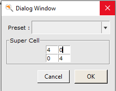
select the Edit → Crystal → Generate Super Cell

go for a 4 by 4 cell as shown below, and press ok.

We have now a bigger slab ready for us putting the CO₂ molecule on.

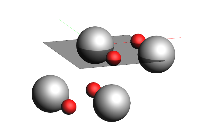
What you need to do next is consider in how many ways can you align a molecule of CO₂ along the MgO surface to create different motifs. We found seven.

Draw a molecule of CO₂

move the whole molecule (hold down the right mouse button) to replicate the following scenarios:

The CO₂ molecule should hover about 2-2.5 Å above the surface (thus, not bonding distance but in the van der Waals catchment area).

Setting up the calculations

We will optimize the first two layers of the slab and the CO₂ molecule and we keep the bottom two layers constraint. This mimics very well what happens on a real surface as only the top layers will react to the adsorbent whereas the bottom layers remain unaffected.

from the Panel bar choose Model → Geometry Constraints and PES Scan

select the bottom two layers of your surface using SHIFT + left mouse button

Press the + next to selected atoms (fix positions)

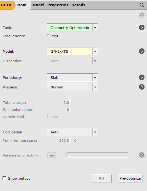
in the main panel

change the calculation setup (Task,**Model**) as follows

The results

Motif by motif look if the calculations converged and if the position of the CO₂ molecule changed. If the latter is the case, you know that your starting position was not close to a favorable minimum. See beyond a discussion of all results and suggestions with what motifs to proceed.

Thus, we will move motifs 1, 3, 4 ,6, and 7 to the next steps.

What to do if my adsorbent is not as simple as CO₂?

CO₂ is very simple to place on an MgO surface as there are not many options. A molecule of glycine would have already many more options as you have a COOH, a CH2 and an NH2 to think about.

As you can see, the more functional groups, the more flexible, the bigger, … the numbers of interaction pattern get out of hand. In this case one could follow the ReaxFF tutorial, Molecular dynamics: Water on an aluminum surface, but use only one molecule of adsorbent. The idea is to perform a molecular dynamic run and check how many motifs, i.e. different alignments of the adsorbent to the surface, you find most often. Extract their geometries and feed into BAND or DFTB and use them as inputs for the workflow discussed in this tutorial.

The adsorption energy

To find out which of the alignment of CO₂ on the surface is the most stable one we have to calculate the adsorption energy, \(E_{ads}\). This energy is a sum of two contributions: the interaction energy, \(E_{int}\), and the distortion energy, \(E_{dis}\).

\(E_{int}\) is obtained as \(E_{motif} − (E_{CO2/motif} + E_{MgO/motif})\). \(E_{motif}\) is the total energy of the whole structure, i.e. slab and CO₂ as calculated in Section 2.2. \(E_{CO2|motif}\) is the total energy of the CO₂ molecule with the geometry it has in the whole structure and \(E_{MgO/motif}\) is the total energy of the MgO slab with the geometry it has in the whole structure. This means we do not consider any deformation; we just want to know the pure interaction energy comprised of electrostatic, dipole, van der Waals interactions, etc.

dissemble each of your motifs:

1. Take the geometry of your motifs and remove the MgO slab

2. Perform a single point calculation* with the same settings on the CO₂ molecule

3. Starting from the full motif structure again:

4. remove the CO₂ molecule

5. Perform a single point calculation with the same settings on the MgO slab

6. Collect the respective Total Energies and calculate \(E_{int}\) as described above

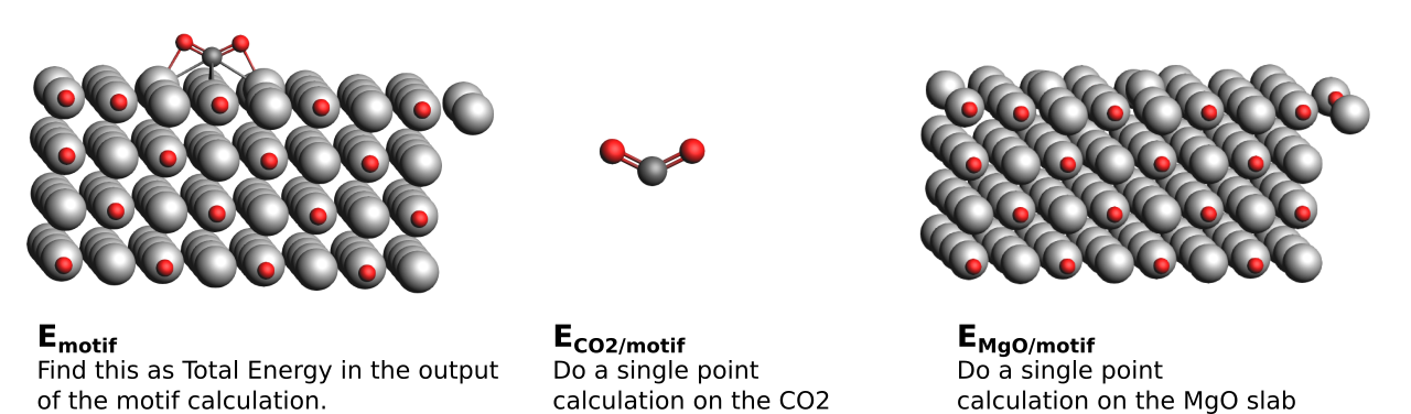
Do this for motifs 1, 3, 4 ,6, and 7.

Motif	\(E_{int}\)	\(E_{motif}\)	\(E_{CO2/motif}\)	\(E_{MgO/motif}\)
1	-5.66	-19434.02743	-311.8223998	-19116.54521
3	-2.67	-19433.79258	-314.0428144	-19117.07485
4	-5.87	-19433.79316	-311.4370726	-19116.48764
6	-0.39	-19431.67584	-314.1733325	-19117.11274
7	-0.34	-19431.62351	-314.1731945	-19117.10762

You can see, purely based on interaction, motifs 1 and 4 have the most favorable interactions.

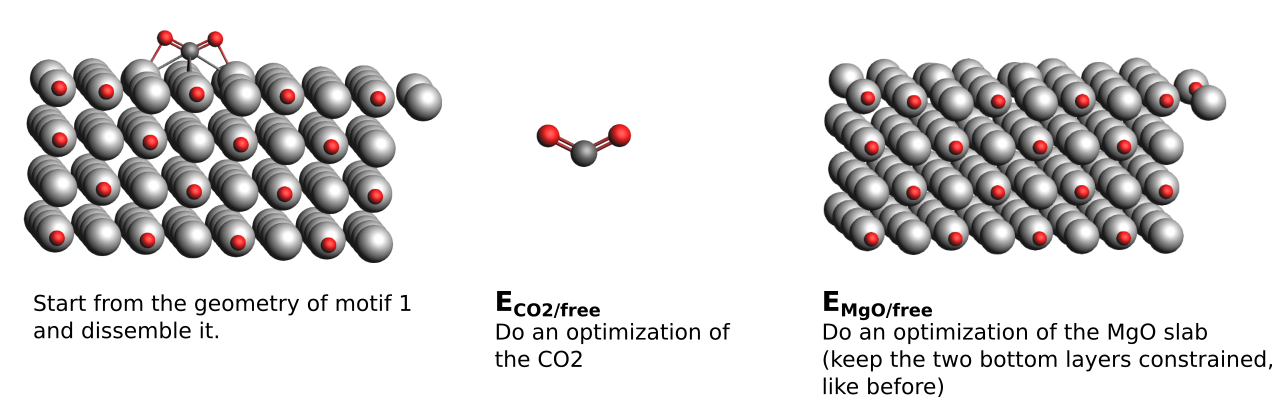
The distortion energy is obtained as \(E_{dis} = E_{MgO/dis} + E_{CO2/dis}\), where \(E_{MgO/dis}\) is the energy to distort the MgO surface from its geometry to that adopted after adsorption and \(E_{CO2/dis}\) is the energy to distort a molecule of CO₂ from its geometry in the vacuum to that one adopted after adsorption. \(E_{MgO/dis}\) is \(E_{MgO/Motif}-E_{MgO/free}\) and \(E_{CO2/dis}\) is \(E_{CO2/motif} - E_{CO2/free}\), respectively.

to calculate \(E_{MgO/free}\) and \(E_{CO2/free}\) you need to dissemble your motifs again:

1. Take the geometry of your motifs and remove the MgO slab

2. Perform a geometry optimization* with the same settings on the CO₂ molecule

3. Starting from the full motif structure again:

4. remove the CO₂ molecule

5. Perform a geometry optimization with the same settings on the MgO slab

6. Collect the respective Total Energies and calculate \(E_{dis}\) as described above

Motif	\(E_{dis}\)	\(E_{MgO/Motif}\)	\(E_{MgO/free}\)	\(E_{CO2/motif}\)	\(E_{CO2/free}\)
1	2.92	-19116.54521	-19117.11603	-311.8223998	-314.1738768
3	0.17	-19117.07485	-19117.11603	-314.0428144	-314.1738768
4	3.37	-19116.48764	-19117.11603	-311.4370726	-314.1738768
6	0.00	-19117.11274	-19117.11603	-314.1733325	-314.1738768
7	0.01	-19117.10762	-19117.11603	-314.1731945	-314.1738768

We can see that motifs 1 and 4 have the highest distortion.

Finally, we can calculate \(E_{ads}\) as sum of \(E_{int}\) and \(E_{dis}\):

Motif	\(E_{ads}\)	\(E_{int}\)	\(E_{dis}\)
1	-2.74	-5.66	2.92
3	-2.50	-2.67	0.17
4	-2.50	-5.87	3.37
6	-0.39	-0.39	0.00
7	-0.33	-0.34	0.01

We can see that Motif 1 has the strongest adsorption energy despite having a very high distortion energy. The latter is outweighed due to the favorable interaction energy as this is the only alignment where all three atoms of the CO₂ molecule are in perfect proximity to the atoms of the MgO surface.