Mechanical properties of epoxy polymers
This tutorial requires the installation of ADF2019 for the calculation of atomic stresses. Details on the calculation of atomic stresses can be found in the ReaxFF manual .
Note
The calculations are computationally demanding. For optimal performance, a parallel execution on a compute cluster is advised. This can best be done by using the remote job management of the GUI
Overview
This advanced ReaxFF tutorial is based on Radue, Jensen, Gowtham, Klimek-McDonald, King and Odegard, J. Polym. Sci. B, 56, 255-264 (2018) [1]. It will demonstrate how to calculate stress-strain curves of an epoxy polymer.
Contents:
- Setting up a strain rate
- Calcuate the atomic stresses
- Results: stress-strain curves, Young’s modulus, yield points…
If you are not familiar with using the GUI yet, you might take a look at the ReaxFF GUI tutorials before continuing.
Tip
The molecular structure used in this tutorial was kindly provided by Matthew S. Radue. Other highly cross linked epoxy polymers can effectively be created with a novel bond boost acceleration method (see tutorial).
Setting up
The polymer used in this tutorial is referred to as Tetra(-epoxy) in [2] since it was build from the tetrafunctional resin epoxy TGDDM (tetra-glycidyl-4,4 0 - diaminodiphenylmethane, Araldite MY 721) and DETDA as hardener. The following cross linking reaction was used to create the polymer structure:

Start by importing the polymer structure into ADFinput
- Click
hereto download the .xyz file tetra_epoxy.xyzImport the coordinates in ADFinput:File → Import Coordinates
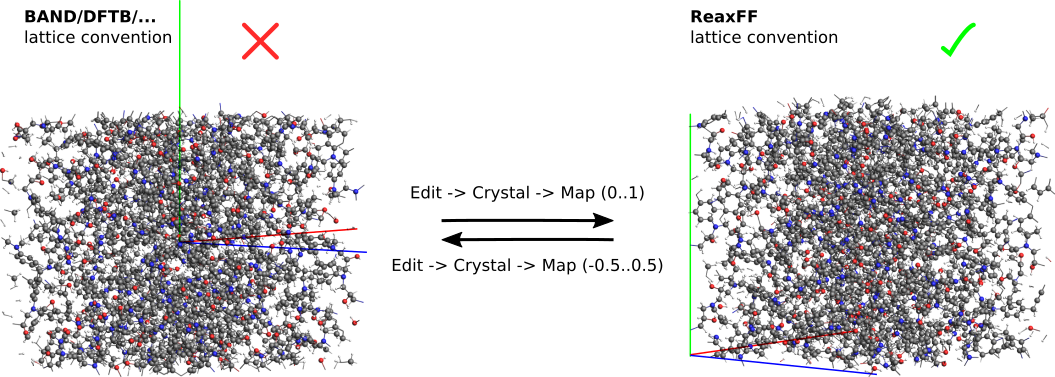
When dealing with periodic systems its always a good idea to take a look at the lattice vectors and check if the ReaxFF lattice convention is applied. If this is not the case, map the coordinates to the ReaxFF unit cell:
Before setting up the strain rate, select 500 ps of NPT dynamics using the following settings
- Force field dispersion/CHONSSi-lg.ffIterations
2000000Method NPT BerendsenTemperature300.15Pressure0.101(1 atm)Damping constant1500.0Stress Stress energy (lstress = 1)

Setting up the strain rate
Strain can be applied with the help of volume regimes in ReaxFF. As in [2] we will use an uni-axial strain, i.e. alongside one lattice vector, and apply a barostat in the lateral directions to account for Poisson contractions.
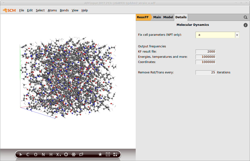
To exclude the direction along which the strain is applied from the barostating
- Go to Details → Molecular DynamicsSelect Fix cell parameters → a
at the same time you can lower the framerate to speed up the calculation and save disc space. For our purposes, writing one frame every 2000 steps (500 fs) is sufficient.
- KF result file:
2000
The ReaxFF volume regimes are expressed as a per-iteration change of a lattice parameter. To display the length of the lattice vectors, go to the lattice panel of the GUI
- Model → Lattice
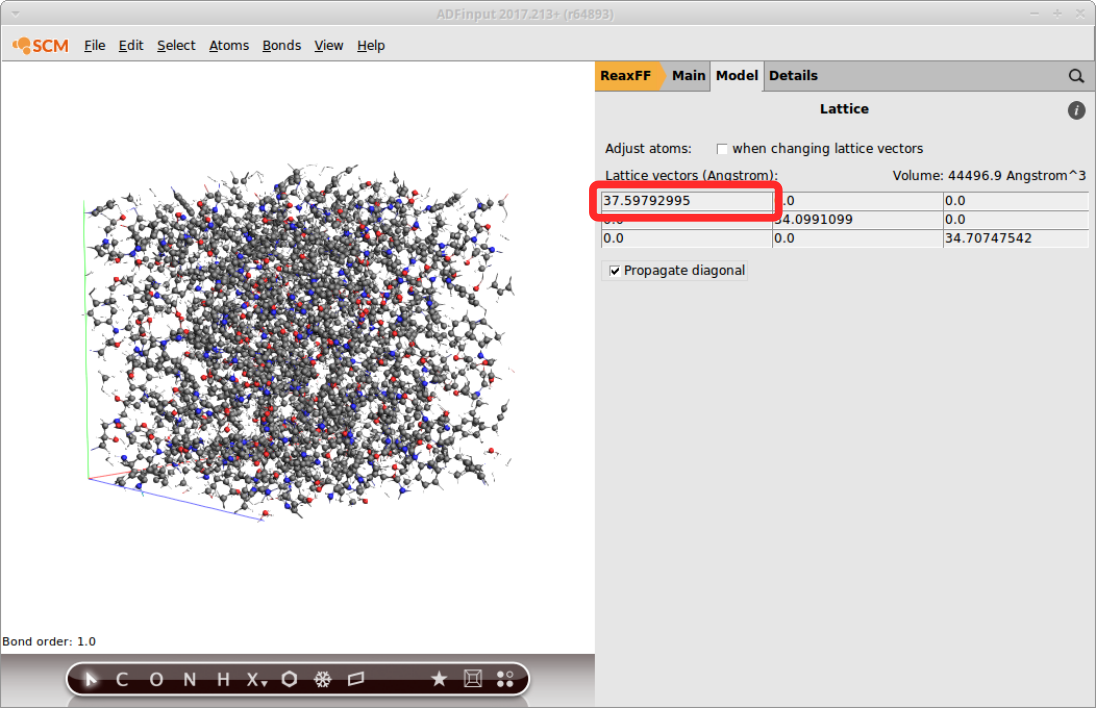
The publication put a strain of 20% over the course of 1 ns. Using the above lattice, and a strain rate of ε = 2 ⋅ 10 -8s -1 the ReaxFF per-iteration volume change ε can be calculated as follows
As a last step, set the according volume regime in the GUI
- Model → Volume RegimePress the + buttonEnter
0.0000019

Note
Remember that the per-iteration change depends on the timestep (0.25fs). Hence: ε iter= 7.52 ⋅ 10 -6/ 4 = 0.0000019
Save the input files with a suitable name, e.g. tetra_strain_a, and run the calculation.
On 16 cores, it will typically take a bit less than 1 day to compute the trajectory depending on your hardware.
Results
Once the calculation has finished, the stress-strain curves can be extracted from the binary results file with the help of a Python script using the PLAMS library.
The script called stress_strain_curve.py is available from here and can be run from the command line:
$ADFBIN/startpython stress_strain_curve.py tetra_strain_a.rxkf
The stress-strain curve is written to a file called stress-strain-curve.csv:
# strain_x, strain_y, strain_z, stress_xx, stress_yy, stress_zz
0.0001 -0.0012 0.0016 -0.0126 0.0107 -0.0142
0.0002 0.0003 0.0025 ...
It can be plotted with any graph plotting software, e.g. gnuplot or qtiplot.
The following example shows how to obtain the mechanical properties from stress-strain plot for an uniaxial strain in y-direction:

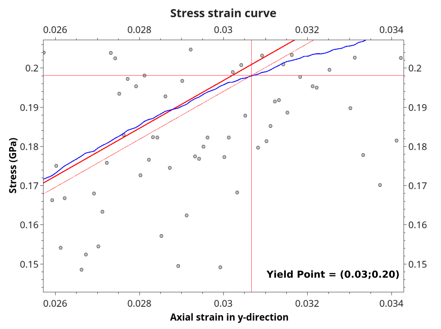
A Young’s modulus of 6.10 GPa was calculated from the slope of a linear fit to the small strain regime (< 0.03). The Yield point is then found as the intersection between the smoothed blue curve (moving window average, 200 points for smoothing) and a 0.2% offset line of the linear fit.
Poisson’s ratio is obtained from the ratio of transverse and uniaxial strains, i.e. plotting column #1 and #3 against column #2 (the system was strained in y-direction)

Since the system is amorphous, Poisson’s ratio becomes (0.54 + 0.20)/2 = 0.37.
Note
In order to get statistically meaningful results, it’s advised to average the mechanical properties, both over different starting structures as well as all three unaxial strain directions. To obtain quality results as in [1], an averaging over 5 different polymer structures using 3 strains each -> 15 trajectories is required.
Lit.:
[1] M. S. Radue, B. D. Jensen, S. Gowtham, D. R. Klimek‐McDonald, J. A. King and G. M. Odegard, Comparing the mechanical response of di‐, tri‐, and tetra‐functional resin epoxies with reactive molecular dynamics, Inc. J. Polym. Sci., Part B: Polym. Phys. 56, 255–264 (2018).