Polymer structures with the bond boost acceleration method¶

In this tutorial we will show how the bond boost acceleration method can be used to drive the non-catalyzed epoxide - amine polymerization reaction with the aim of generating highly crosslinked epoxy polymer structures:

Fig. 10 Epoxide - amine polymerization reaction

The goal is not to capture or simulate the kinetics of the polymerization reaction, but rather to generate realistic atomistic models of epoxy polymers which can used in further simulations (e.g. for prediction of mechanical properties)

This advanced ReaxFF tutorial is loosely based on the following publications:

This tutorial requires the installation of AMS2019 for the bond boost acceleration method.

If you are not familiar with using the GUI yet, you might take a look at the ReaxFF GUI tutorials before continuing.

More details and information on other acceleration methods can be found in the ReaxFF manual:

Tip

See also the tutorial Mechanical properties of epoxy polymers

Setting up¶

The cross linking polymerization reaction occurs between the epoxy and the amine groups. The reaction is depicted in its simplest, non-catalyzed form in Fig. 10.

Throughout this tutorial the epoxy resin will be BisF whilst DETDA will be used as the hardener (amine):

You can either draw the 3D structures of these molecules with the GUI or download the xyz files:

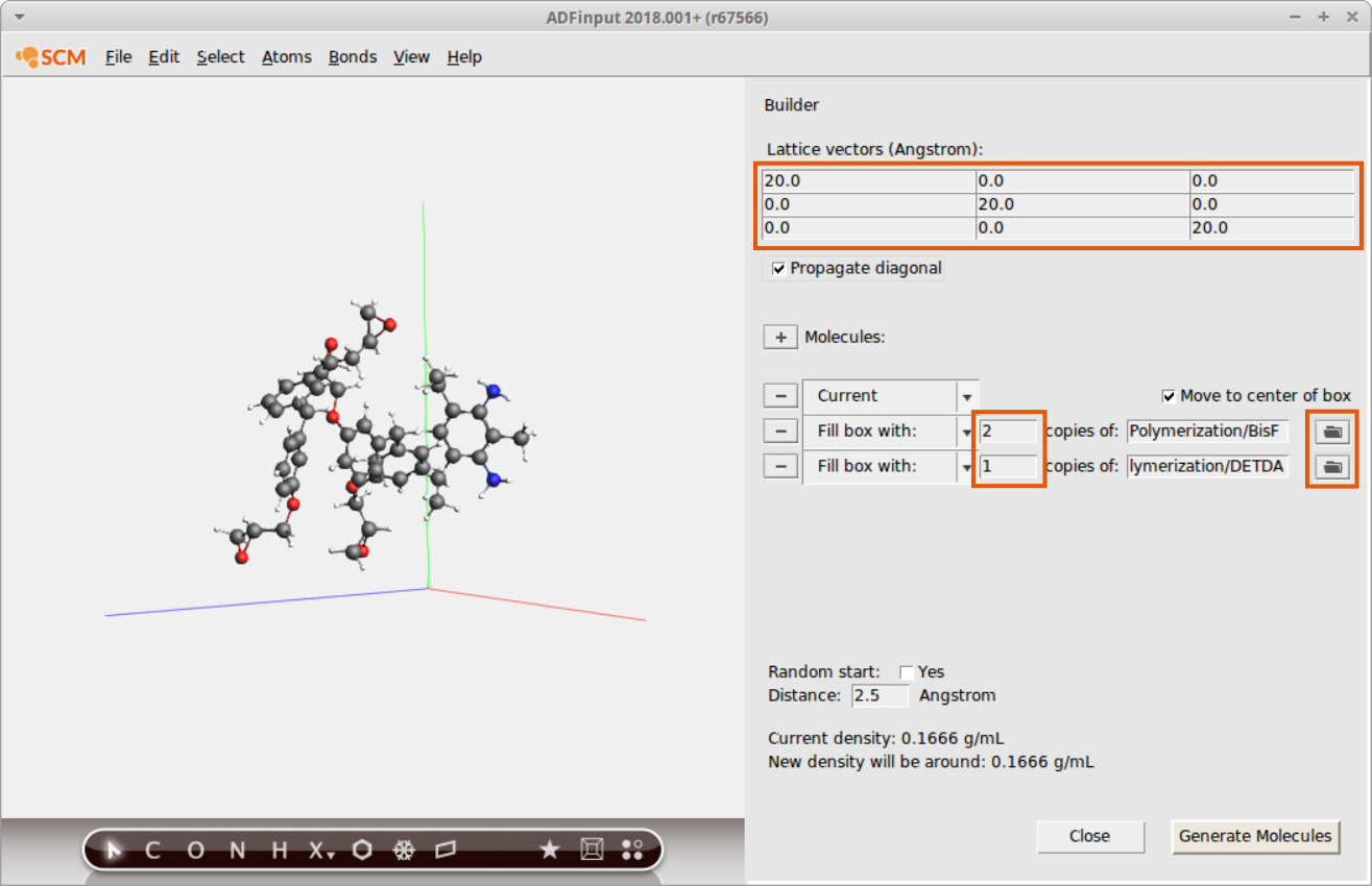
: Click to download here to download the .xyz file BisF.xyz

Click to download here to download the .xyz file DETDA.xyz

Use the builder functionality in ADFinput to fill a periodic box with one DETDA and two BisF molecules:

: Go to Edit → Builder to open the Packmol dialog

Enter 20, 20 , 20 on the diagonal for the lattice vectors

Click on the Folder icon and select the file BisF.xyz you just downloaded

Click on + button and open the file DETDA.xyz

Enter 2 and 1 for BisF and DETDA respectively

Click on Generate Molecules

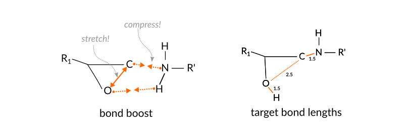
To accelerate a reaction with the bond boost method, ReaxFF needs to be provided with a set of atom distances that define a preliminary complex which could lead up to the transition state of the reaction. If this complex is formed during the dynamics, external forces are applied to support bond breaking and bond formation for a user defined set of bonds. This ‘boost’ lasts for user defined time during which the reaction may or may not occur.

For the current reaction, a simple, yet effective set of atom distances are those between the N atom and the terminal C-atom of the epoxy group as well as the distance between the O-atom of the epoxy group to whichever H-atom of the amine group is closest:

It is possible to distinguish atoms depending on their chemical environment, e.g. the terminal C-atom of the epoxy group, but the information needs to be provided via the regions model of ReaxFF by the user. To distinguish the terminal C-atom from all other C-atoms in the system, a CT region needs to be setup:

: Go to Model → Regions

Click + button next to Regions on the top

Enter a suitable name for the new region CT

Select a terminal C-atom in the molecule panel

Click on the + button next to the CT region

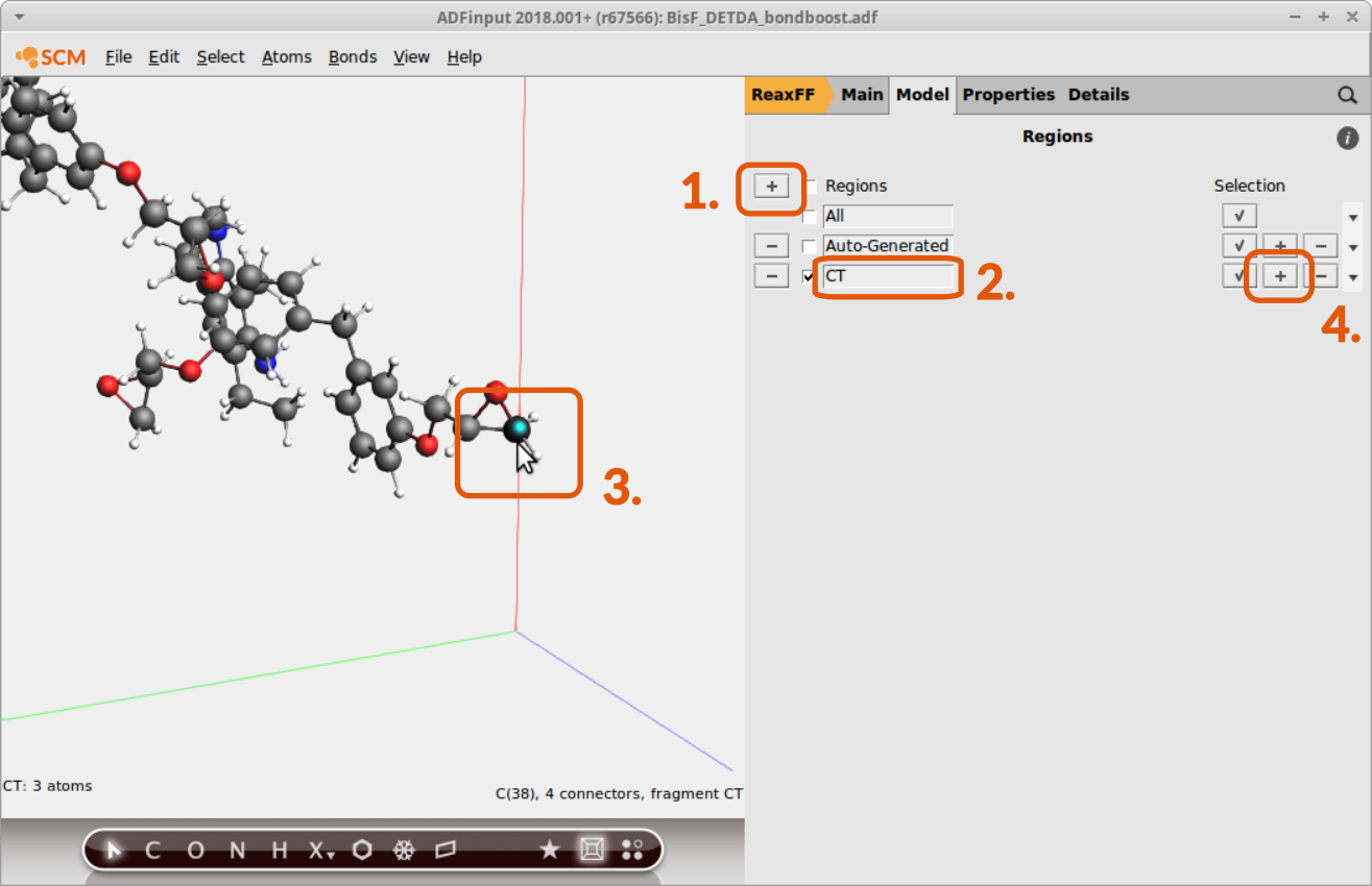
Repeat steps 3. and 4. to add all other terminal C-atoms to the new CT region

Tip

You can hold down the SHIFT key to select multiple atoms in the molecule view.

Tip

If you have multiple identical molecules, the region can be copied over in the Regions panel using the ‘Apply To Identical Molecules’ option from the dropdown menu on the right.

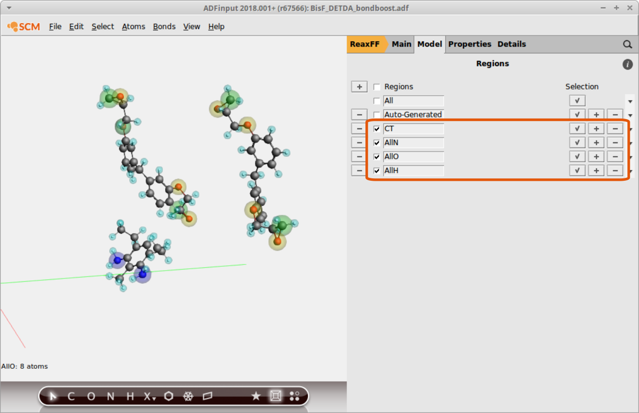
Now the subset of terminal C-atoms can be distinguished via referring to the region CT as we’ll see later. The other regions are consisting of all N-,O- and H-atoms. To set up a region with all N-atoms:

: Create a new region: Click + button next to Regions

Enter a suitable name: AllN

Select one N-atom

Go to Select → Select Atoms Of Same Type

Click on the + button next to the AllN region

Tip

Make sure that the atoms of the previous region assignment are not selected anymore when assigning a new region. Trying to assign one atom to multiple regions is a common source of error.

Continue setting up regions containing all O- and H-atoms respectively:

Once the regions are set up, we can use them to define a tracking regime for the bond boost. The set of atom distances that will switch on the boost once all criteria are met is

to set this up in the GUI

: Go Model → Bond boost

Click on the + button next to Detect initial configuration

From the Atom types dropdown menus, select AllN and C-CT

Set Rmin and Rmax to 3.0 and 7.0 respectively

Continue with assigning the other tracking options:

C-CT / O-AllO 1.2 - 3.0
O-AllO / H-AllH 3.0 - 8.0
H-AllH / N-AllN 0.8 - 1.5

../_images/bond_boost_tracking_gui_2.png

The boost settings are chosen such that the following logic is implemented

the aim is to support the breaking and forming of bonds but still allow the reaction to fail.

Note

The above settings have been chosen empirically. A more thorough assessment of energetics based on ab initio calculations is presented in the publication by A. Vashisth et al.

The bond boost options are defined in the lower part of the bond boost panel

: Click on the + next to Add boost

Choose the atoms N and C from the dropdown menu

Set R₀(target bond length) to 1.5

Set the force constants F₁ and F₂ to 400.0 and 0.75

Continue with assigning two more boosts:

3:O / 4:H 1.5 , 300.0 , 0.50
4:C / 5:O 2.5 , 100.0 , 0.75

Running and analyzing¶

After completing the setup of the bond boost in the previous chapter, we can test the boost by running a small NVT trajectory. Choose the following general ReaxFF settings from the main panel

: Force field dispersion/CHONSSi-lg.ff

Temperature 500.0

Save and Run

../_images/bond_boost_trajectory_settings.png

Note

This tutorial employs the dispersion corrected force field, that has not been optimized for usage with the bond boost. This force field has been used successfully in the study by M.S. Radue et al. The results might be improved by using the force field CHON2017_weak_bb.ff fitted for usage with the bond boost method (A. Vashisth et al. ). However, note that switching the force field will require tweaking the bond boost settings.

Open ADFmovie and follow the calculation of the trajectory, you should see at least one successful cross linking reaction. The total amount of cross-linking reactions can be somewhat estimated by displaying the number of molecules:

: Properties → Number of Molecules

Polymerization workflow¶

A high throughput screening of epoxy polymers constructed from different resin-hardener combinations requires automation of the following steps:

packing of a random start periodic box
running bond boost trajectories
equilibrate the polymers using NPT dynamics

By employing random starting conditions the workflow should be able to produce different polymer structures that can be used for averaging when the quantity of interest. e.g. Young’s modulus, is calculated.

The workflow presented here has been written in Python and makes use of the PLAMS library. It can be executed as is with the plams interpreter that is shipped with any ADF install.

A complete package containing the scripts and input files is available for download from here In the following the single steps of the workflow are explained in more detail. If you just want to try and run the workflow, you can just execute the script:

: Download the workflow package from here

move into a suitable location, e.g. the ADF_DATA folder on windows

from inside the folder EPOXY-POLYMERIZATION run the command: $ADFBIN/plams ./scripts/bond-boost.py

This will generate five small epoxy polymers from 8 BisF and 4 DETDA molecules:

Note

On a windows machine make use of the pre-configured command line, adf_command_line.bat as described in the scripting documentation

Description of the workflow¶

1. Generating random start structures

The generation of a random starting structure is achieved by the following approach: Based on a user specified ratio of resin:hardener, the resin and hardener molecules are placed on a regular grid with the help of utility script pack-box.py (see below for details on how to use your own molecules).

The polymerization workflow in bond-boost.py will then employ a simulated annealing run to generate a random structure out of this regular molecular crystal:

The total number of steps for this annealing run are set to a default of 100 000 within the file bond-boost.py

# how much MD steps for the sim. annealing?
sim_annealing_steps = 100000

the temperature program is defined inside the corresponding tregime.in file. The example uses the file tregime_TGAP.in:

#Temperature regimes
#start #nzones at1 at2 T1 Tdamp1 dT1 ...
0 1 1 941 298.0 100.0 0.0125
25000 1 1 941 600.0 100.0 0.0
75000 1 1 941 600.0 100.0 -0.0125

Starting from 298.0K the system is heated up to temperature of 600K and kept there 50000 steps before cooling down to room temperature with the same rate again. The results of this calculation are found in the plams results folder, inside the folder entitled SimAnnealing_orig-TGAB_DETDA_2.

2. Running the 1st bond boost

We found that running a preliminary boost in which only half the possible cross linking reactions is boosted, supports the formation of polymer structures with higher cross linking ratios. The easiest way to do so is, to assign two different regions to the N-atoms of the hardener, i.e. N1 and N2.

For the workflow this means only N-atoms that belong to the region N1 are affected by this first bond boost calculation:

The settings for this step can be found in the file bond-boost.py

# how much MD steps for the 1st boost?
first_boost_steps = 100000
# temperature during the 1st boost?
first_boost_temp  = 500

the settings for the bond boost method are found in the file ./orig/tracking.in:

# Distance regimes
# T pair1: at1 at2 min max  pair2: at1 at2 min max  pair3: at1 at2 min max  pair4: at1 at2 min max  pair5: at1 at2 min max
4    N1 C2 3.0 7.0    C2 O 1.2 3.0    O H 3.0 8.0    H N1 0.8 1.5
# Restraint settings
# iter nr. r1: at1 at2  R0   F1   F2  r2: at1 at2  R0   F1    F2  r3: at1 at2  R0   F1    F2  r4: at1 at2  R0   F1   F2
10000 3    1 2 1.5 400.0 0.75    3 4 1.5 300.0 0.5    2 3 2.5 100.0 0.75

A good way to follow the progress is to open the trajectory found in the folder plams*/boost… with ADFmovie and display the total number of molecules (Properties → Total Number of Molecules):

../_images/bond_boost_wf_visualize_boost.png

This will only show cross linking reactions that reduce the total number of molecules but this is true for the majority of reactions in the first stage.

3. Running the bond boost and compressing the box

In this stage all constraints on the bond boost are dropped by taking the geometry resulting from the previous bond boost run and changing those atom labels reading N2 to N1. With the tracking options remaining unchanged, all cross-linking reactions involving the N-atoms of the hardeners will be boosted.

At the same time, a compression regime is used that slowly shortens all three lattice vectors of the periodic cell until the target density, e.g. 1.2 kg/l, is reached. The default compression rate applied is -0.0001 Å / Iteration. Every 20 000 iteration the structure is subject to a geometry optimization with fixed lattice vectors to account for relaxation processes. The compression/geo-optimization step is repeated until a maximum number of iterations or the target density of the polymer is reached.

../_images/bond_boost_wf_compression.png

Note

Running NPT dynamics to equilibrate the polymer structure to atmospheric pressure will have the same effect but takes much, much more time to equilibrate. Note that M.S. Radue et al used a compression scheme in their study as well. Of course the structures generated by this workflow should be equilibrated before production use, e.g. for the prediction of mechanical properties.

The settings for this steps can be found in the bond-boost.py file

# How much MD steps before GeoOpt?
md_steps_before_geo_opt = 20000

# Thermostat
second_boost_temp  = 500

# Stop workflow at this target density
target_density = 0.5 # kg/l

# how much geo opt iterations?
max_opt_steps = 100

# maximum number of iterations (if density criterion isn't fulfilled)
max_iterations = 15

4. Analyzing the results

Take a look at the logfile called boost.log to see in which folder the final structures can be found. For example, the following lines:

MD_1_1 orig-BisF_DETDA Density: 0.27 (Target Dens.: 1.20) [kg/l]
MD_1_2 orig-BisF_DETDA Density: 0.39 (Target Dens.: 1.20) [kg/l]
MD_1_3 orig-BisF_DETDA Density: 0.58 (Target Dens.: 1.20) [kg/l]
MD_1_4 orig-BisF_DETDA Density: 0.91 (Target Dens.: 1.20) [kg/l]
MD_1_5 orig-BisF_DETDA Density: 1.58 (Target Dens.: 1.20) [kg/l]
-----------------------------------------------------------------------
FINAL: MD_1_5 orig-BisF_DETDA Density: 1.58 (Target Dens.: 1.20) [kg/l]
-----------------------------------------------------------------------

indicate that the polymer created from TGAP and DETDA (from the example calculation) reached the target density during the MD run labeled MD_1_7. The trajectory is then located in the folder plams.10547/MD_1_7/MD_1_7.kf The naming of the PLAMS results folder will be different with each run, ensuring unique naming, even in the case of a complete rerun.

Cross linking ratios can be calculated via a script called cross_linking_ratio.py found in the folder scripts. Execute the script as follows from where this README file is located:

$ADFBIN/startpython scripts/cross-linked-density.py plams.10547/MD_1_7/MD_1_7.kf

the max. cross linked density will be calculated on printed on the screen. The temporal evolution of the cross-linking is written to a file called cross-linked-density.out.

Note

The python script used for the calculation of cross linking ratios uses the atom types defined in the force field. If used with a different force field than dispersion/CHONSSi-lg.ff, those need to be adjusted in the top line of the script.