Vibrationally resolved electronic spectra of naphthalene
In this tutorial we use the vertical gradient Franck-Condon (VG-FC) Vibronic-Structure Tracking (VST) method to calculate the vibrationally resolved absorption spectrum of the first excited singlet state of naphthalene.
There are different methods to calculate a vibrationally resolved absorption spectrum. Out of these methods VST is in principal the quickest method and can also be used for much larger sized molecules. It is based on a mode-tracking algorithm and works by tracking those modes that are expected to have the largest impact on the vibronic-structure of the spectrum. Note that VST is not supported by the standalone ADF program, we need the so called AMS driver. Note that the overhead of running ADF through AMS is relatively large. More information on VST and related methods can be found in the AMS user manual:
Step 1: Geometry Optimization
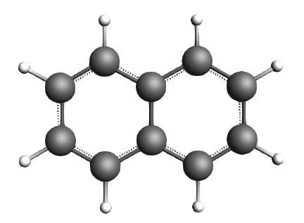
Let us first obtain a naphthalene molecule, and optimize its geometry with ADF.
- Start ADFJobs.Click on SCM → New Input. This will open ADFInput.In ADFInput, click the search icon
 and type “naphthalene” into the box.Select the “Naphthalene (ADF)” entry from the molecules section.Click the Symmetrize button
 to check the symmetry (should be D2h)Select Task → Geometry Optimization.Select Frozen core → None.Click on File → Save As… and give it the name “naphthalene_GO”.Click on File → Run.Wait for the calculation to finish.Click “Yes” when asked to read new coordinate
Step 2: Excited state gradient
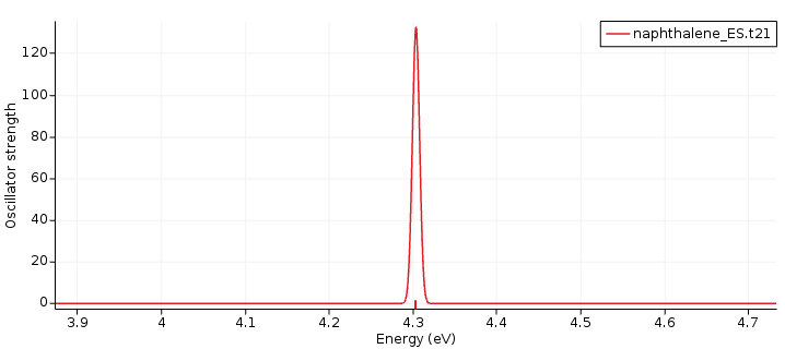
Here we will look at the vibrationally resolved absorption spectra of the lowest electronically excited singlet state S1. The VG-FC Vibronic-Structure Tracking method needs the excited state gradient of S1 at the ground state geometry.
- Select Task → Single Point.Panel bar Properties → Nuclear Gradients.Check the Calculate Gradients checkbox.Panel bar Properties → Excitations (UV/Vis), CD.Select Type of excitations → SingletOnly.Enter ‘1’ for Number of excitations.Panel bar Properties → Excited State Geometry.Check the All Gradients checkbox.Click on File → Save As… and give it the name “naphthalene_ES”.Click on File → Run.Wait for the calculation to finish.Click on SCM → Spectra.Axes → Horizontal Unit → eV.Width → 0.01.
Step 3: Vibronic-Structure Tracking
The calculated lowest excited singlet state is of B2.u symmetry. For the VG-FC vibronic-structure tracking method we need a new input, in which we will use ADF as an AMS engine.
- Click on SCM → New Input.Click on File → Import Coordinates… and and select the “naphthalene_ES.adf” file.Select the ADF via AMS panel:
 →
→  .Select Task → Vibrational Analysis.Select Frozen core → None.Panel bar Model → Vibrational Analysis.Select Type → Vibronic Structure Tracking.Panel bar Details → Vibrational Analysis Excitation.Click on the folder next to Excitation file: and select naphthalene_ES.t21Enter ‘B2.u 1’ for Singlet.Panel bar Details → Vibrational Analysis Spectrum.Enter ‘50’ for Line width in cm-1.Click on File → Save As… and give it the name “naphthalene_VST”.Click on File → Run.Wait for the calculation to finish (may take several minutes).Click on SCM → Spectra.
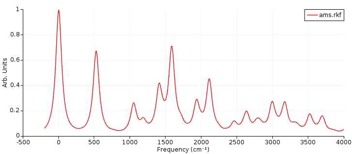
The spectrum is relative to the 0-0 excitation energy. The default (artificial) broadening is relatively wide, therefore it was changed to 50 cm-1.