Benzene molecule in a magnetic field
This tutorial will show you how to:
- handle the effect of a magnetic field on a molecule using BAND
- visualize the resulting vector field (magnetic current) as vectors, and as streamlines
Step 1: adfinput
Start ADFinput in a clean directory. (according to Step 1 of the Getting Started with BAND)
Step 2: Setup the system - benzene
Make a benzene molecule. One easy way is to search ( ) for Benzene and select it.
- 1. Make a benzene molecule.
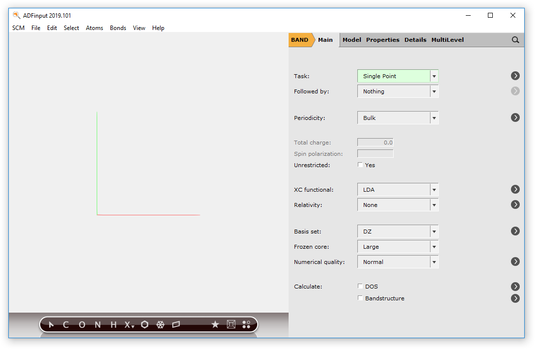
Go to the Main panel for BAND, and turn of periodicity:
- 2. Switch to BAND:
 →
→  3. Periodicity None

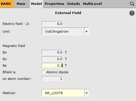
and turn on the magnetic field:
- 4. Go to the External Field panel.5. Enter 0.1 in the Bz field.6. Select the NR_LDOTB method.
Step 3: Run the calculation
Now you can save and run the calculation.
- 1. File → Save, give it a name and press Save.2. File → Run
Step 4a: Magnetic current: vectors
After the calculation finished, open the result file with ADFview:
- 1. SCM → ADFview
Add a vector field:
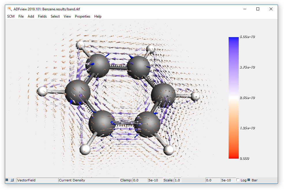
- 2. Add → Vector Field3. Select the Magnetic and Current fields → Current Density
You will not see any vectors yet. The reason is that the vectors are very small. If you move the mouse over the real field at the bottom right (the max-color field), you can notice the range in the help balloon.
The vectors in the Clamp range will be scaled to vectors in the 0 .. 1 range. To make our vectors visible, change the upper clamp value to a smaller number:
- 4. Change the second clamp value to 5e-105. Change the color max value also to to 5e-106. Check the box in front of Bar to show the color bar7. Rotate and zoom the image to get a good view
Now you should see your vector field similar to this:
If you wish you can play with the values in the control line. Please use the help balloons, the meaning of those values is not obvious!
Step 4b: Magnetic current: streamlines
Another way to visualize a vector field is to generate streamlines.
Conceptually, one defines seed points, and then a line is generated starting at each seed point, following the vectors. For visualization purposed, a tube is generated around the lines, and the width of the tube depends on the magnitude of the vectors.
There are many options, the most important is to select the seed points. Again, the help balloons are important, they describe in detail what the controls do.
The default is to use starting points randomly distributed in a sphere:
- 1. Add → StreamLines2. Select the Magnetic and Current fields → Current Density3. Change Npts to 154. Change R to 55. Change the max-color field to 5e-10

An alternative is to define a line, and generate the starting points linearly distributed along that line. You can activate controls for the line to position it as you want.
- 6. Change Sphere to Line7. Check the Controls box8. Drag the end points of the line such that the line crosses the benzene diagonally (out of plane)
Finally you can use a grid in a plane as starting points for the streamlines. Npts is the number of grid lines per dimension, thus the number of streamlines will be the square of Npts if you are using a plane.
The StreamLines technique has some important Detail options. To get them, select the Show Details option from the StreamLines pull-down menu at the bottom. The help balloons give the details, especially the streamline radius and the scaling method (flux or norm) are important.
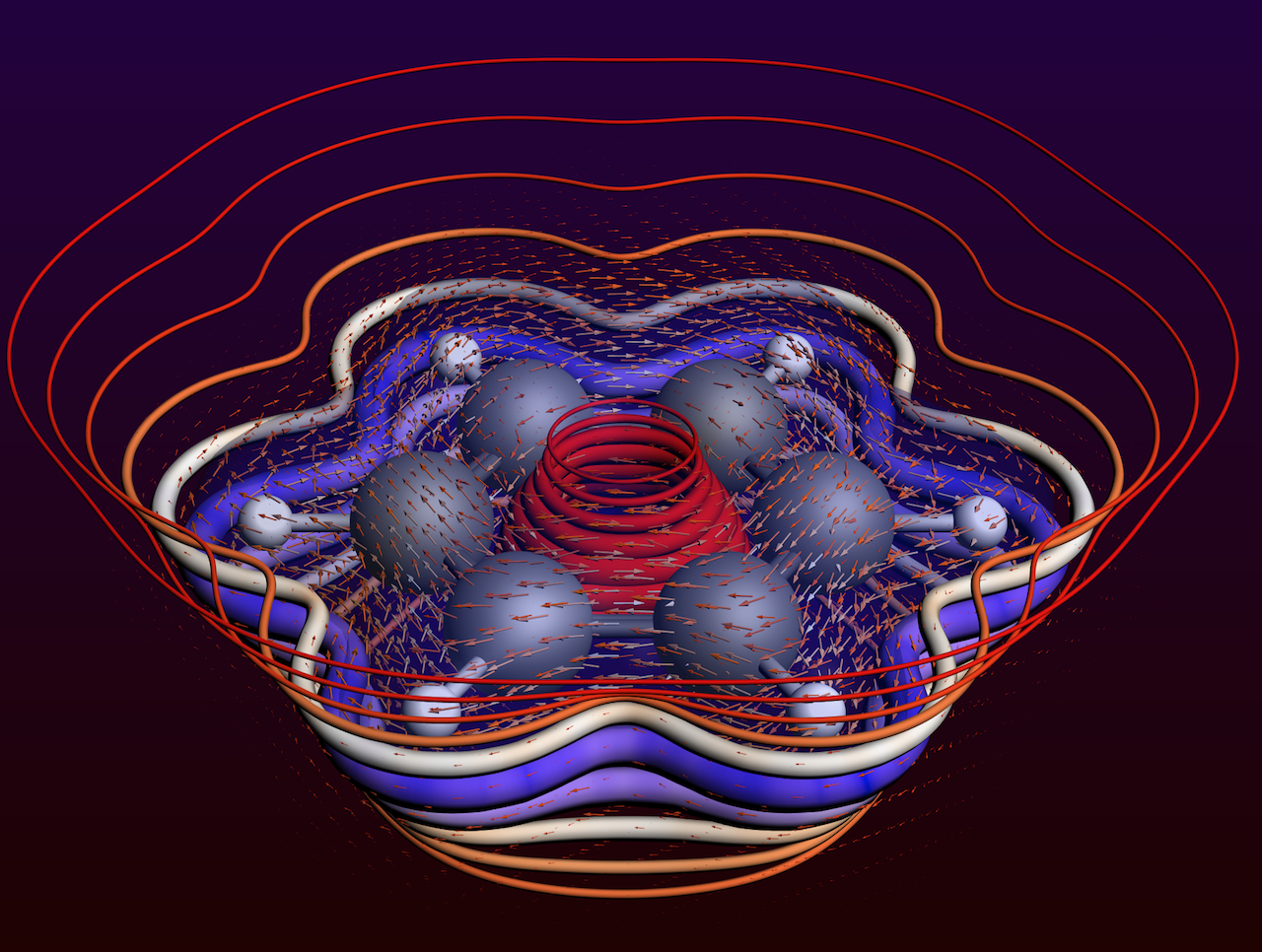
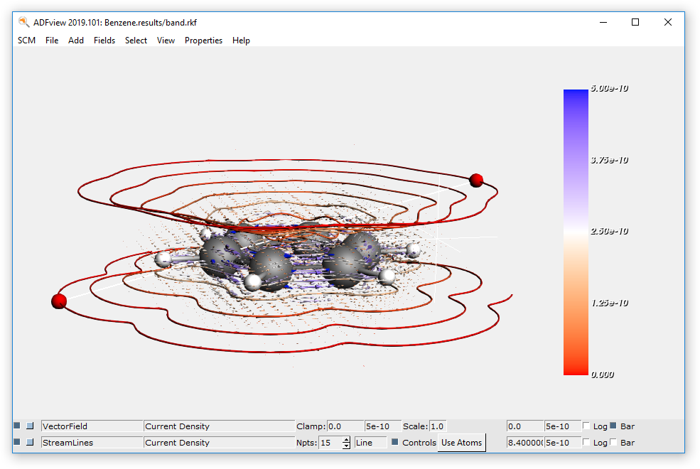
Now try for yourself, make some nice looking picture… the following was made combining several techniques from above.
- 9. Experiment, try to make a picture similar to the following picture.Hint: it consists of vectors visualization, and TWO sets of streamlines (and an improved background color).