Overview: parameters and analysis
Step 1: Start ADFcrs
For this tutorial it is convenient to start with an empty directory, for example, with the name Tutorial. You should start ADFjobs and move to the Tutorial directory:
- Start adfjobsClick on the Tutorial folder iconSelect SCM → COSMO-RS

This ADFcrs window consists of the following main parts:
- the menu bar with the menu commands
- on the left: a list of compounds and the possibility to add compounds
- on the right: some properties for the selected compound
This is the so called List of Added Compounds, which is the window you will get if you select Compounds → List of Added Compounds.
If you run the COSMO-RS GUI the first time, you will be asked if you would want to download and install the COSMO-RS compound database:

If you have the permission to write such directory (typically in $ADFHOME/atomicdata/ADFCRS-2018), it is recommended to download this COSMO-RS compound database. You may need to have administrator privileges to do so. On the other hand, for this tutorial, it is not necessary that the COSMO-RS compound database is downloaded.
Step 2: Add Compounds
In tutorial 1 it was shown how to make ADF COSMO result files. In this tutorial we will use some ADF COSMO result files that were made before. These files can be found the directory $ADFHOME/examples/COSMO-RS/Parameters_and_Analysis. Copy these COSMO result files (water.coskf, methanol.coskf, ethanol.coskf, and benzene.coskf) to the directory Tutorial. As the name suggests these are COSMO result files of water, methanol, ethanol, and benzene, respectively.
Note that these COSKF (.coskf) files contain only the part of an ordinary TAPE21 (.t21) file which is needed in a COSMO-RS calculation. These COSKF files can only partly be used in ADFview, for example.
- Press ‘Add’ for ‘Add Compound(s)’ in the left window

A file select box will open, that looks like (may look different on different platforms)

or

- Select Files of type (or Filter) → COSMO kf file (*.coskf)Select multiple files: benzene.coskf ethanol.coskf methanol.coskf and water.coskfClick ‘Open’
On the right side of the List of Added Compounds one finds some data that was written from the last file that was opened, in this case water.coskf. Here it is also possible to add some pure compound input data. We will not do so now since there is no need. For some other types of compounds user input is required at this point, however. We will encounter an example of that in the next step.

Step 3: Set pure compound parameters
In the COSMO-RS model [1] there is a ring correction term. This is important for, for example, the benzene molecule, which has 6 ring atoms. However, it is really required only when the vapor pressure of the compound is going to be computed (either because that is explicitly requested or because it is used in predicting partial vapor pressures in a mixture or gas/liquid partitioning coefficients).
For some properties, like solubility of a solid, one can or one has to include some pure compound properties in the left window of the List of Added Compounds for a selected compound.
It is possible to save this pure compound data in as a new COSKF file (or COSMO file).
- Click in the left window (in the List of Added Compounds) benzenePress ‘Generate’ for ‘Nring’ in the right window

To save this data in a .coskf file
- Click in the left window (in the List of Added Compounds) benzenePress ‘Save As’ at the top of the right windowEnter the name ‘benzene’ in the ‘Filename’ field
If you have followed this tutorial from the start then you will overwrite an existing benzene.coskf file. You will be asked if you want to to that, click ‘Yes’. The writing can take some time, especially for larger compounds. During this time the COSMO-RS GUI is not available for other actions.
Notice that there are ‘Estimate’ buttons to estimate some pure compound properties. The method that is used for the estimation is a group contribution method. If one Presses all ‘Generate’ and ‘Estimate’ buttons one could get something like the next for benzene

Note that some of the estimates are not so good, like the estimated melting point of small molecules.
Step 4: COSMO-RS, COSMO-SAC, and UNIFAC parameters
One can easily change between the COSMO-RS, COSMO-SAC, and UNIFAC method that is going to be used in the calculation by selecting Method → COSMO-RS, Method → COSMO-SAC, or Method → UNIFAC. Here we will use COSMO-RS, since ADF was parametrized for this method.
- Select Method → COSMO-RS
Expert option: set COSMO-RS parameters
- Select Method → COSMO-RSSelect Method → Parameters

Default ‘ADF combi2005’ COSMO-RS parameters are selected, which are ADF optimized COSMO-RS parameters. See also a discussion of the COSMO-RS parameters in the COSMO-RS manual. If one selects the ‘Klamt’ option for ‘Use: … COSMO-RS parameters’, the optimized parameters are chosen, which are optimized by Klamt et al., see ref. [1].
Expert option: set COSMO-SAC parameters
- Select Method → COSMO-SACSelect Method → Parameters

The 2013-ADF COSMO-SAC parameters were optimized for use with ADF. See also a discussion of the COSMO-SAC parameters in the COSMO-RS manual.
Expert option: set UNIFAC parameters
- Select Method → UNIFACSelect Method → Parameters
No screen shot is given, since at the moment one can not choose different sets of UNIFAC parameters. Only the so called original UNIFAC parameters are implemented.
The UNIFAC implementation needs a SMILES string to generate the groups in a compound. The generation of SMILES strings is not done automatically.
- Click in the left window (in the List of Added Compounds) waterPress ‘Generate’ for ‘SMILES’ in the right windowClick in the left window (in the List of Added Compounds) ethanolPress ‘Generate’ for ‘SMILES’ in the right windowClick in the left window (in the List of Added Compounds) methanolPress ‘Generate’ for ‘SMILES’ in the right windowClick in the left window (in the List of Added Compounds) benzenePress ‘Generate’ for ‘SMILES’ in the right window
For example, for benzene, the SMILES string ‘c1ccccc1’ should be generated (by Openbabel). One should check the SMILES string generated, especially for charged systems, radicals, and anorganic compounds.

For the rest of the tutorial the COSMO-RS method will be used:
- Select Method → COSMO-RS
Step 5: Visualize the COSMO surface: ADFview
You can use ADFview to have a look at the COSMO surface, and the COSMO surface charge density. This is possible if the COSMO result file of the compound is a .coskf file or a .t21 file.
- Select Compounds → List of Added CompoundsClick on the left side waterPress on the right side ‘Show 3D’An ADFview window should pop-upSelect ADFview → Add → COSMO: Surface Charge Density → on COSMO surface (reconstructed)Select ADFview → View → Background → WhiteIncrease the size of the ADFView window,such that a control line at the bottom of the ADFview window is visibleIn the control line click on the ‘Cosmo surface’ pull-down menu and use the Show Details commandSelect in the lowest line Colormap → RainbowIn the control line click on the ‘Cosmo surface’ pull-down menu and use the Hide Details command
Then you will see something like:
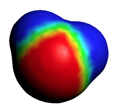
The red part represents positive COSMO charge density (the underlying molecular charge is negative), the blue part negative COSMO charge density (the underlying molecular charge is positive). You can also look at the COSMO surface points themselves.
- Select Add → COSMO: Surface Charge Density → on COSMO surface pointsIn the control line click on the ‘Cosmo surface points’ pull-down menu and use the Show Details commandSelect Colormap → RainbowIn the control line click on the ‘Cosmo surface points’ pull-down menu and use the Hide Details command

The small spheres represent the COSMO surface points that are used for the construction of the COSMO surface.
Next we will close this ADFview window.
- Select the ADFView window ‘water’Select File → CloseSelect the COSMO-RS GUI window
ADFview has many options to change the look of the picture.
- Select Compounds → CompoundsClick on the left side methanolPress on the right side ‘Show 3D’An ADFview window should pop-upSelect ADFview → Add → COSMO: Surface Charge Density → on COSMO surface (reconstructed)Select ADFview → View → Background → WhiteCheck ADFview → View → Anti-AliasIncrease the size of the ADFView window, such that a control line at the bottom of the ADFview window is visibleIn the control line click on the ‘Cosmo surface’ pull-down menu and use the Show Details commandChange the Opacity to 70Select Colormap → Rainbow

Next we will close this ADFview window.
- Select the ADFView window ‘methanol’Select File → CloseSelect the COSMO-RS GUI window
Optionally one can change the default settings for the colormap that is used in ADFview
- Select SCM → Preferences → Module → ADFviewSelect Colormap → Rainbow
Step 6: Analysis: The sigma profile
The \(\sigma\)-profile shows the amount of surface area for a given COSMO charge density.
- Select Analysis → Sigma Profile Pure CompoundsCheck the ‘+’ button to add ‘benzene’, ‘ethanol’, ‘methanol’, and ‘water’
- Select File → Save AsEnter the name ‘tutorial2’ in the ‘Filename’ fieldSelect File → Run
The sigma profiles (\(\sigma\)-profile) of the four pure compounds will be shown in a graph and in a table in the right part of the window. The whole window can be resized. The relative size of the left part of the window compared to the right part can be changed if one moves the sash that is in between these parts. In the right part of the window one can also change the relative size of the upper part compared to the lower part if one moves the sash that is in between these parts.

With default settings, if one clicks in the graph one can zoom (right mouse, or Command-Left (drag up or down)), or translate (left mouse) the graph. If one clicks in the graph window at the left or below the axes, a popup window will appear in which one can set details for the graph window.
Note that the \(\sigma\)-profile depends on the method (COSMO-RS or COSMO-SAC) that was used in the calculation. Here we have used COSMO-RS. In this case the \(\sigma\)-profile depends on the actual value for r_av (rav ), which is one of the COSMO-RS parameters, see one of the previous steps.
One can also look at the hydrogen bonding part of the \(\sigma\)-profile.
- Select Graph → Y axes → hydrogen bonding (HB) part sigma profile

Step 7: Analysis: The sigma potential
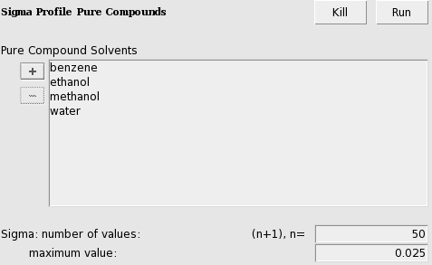
- Select Analysis → Sigma Potential Pure CompoundsCheck the ‘+’ button to add ‘benzene’, ‘ethanol’, ‘methanol’, and ‘water’Press ‘Run’
The sigma potentials (\(\sigma\)-potential) of the four pure compounds will be shown in a graph and in a table in the right part of the window. The \(\sigma\)-potential depends on the temperature of a compound. Here the temperature is set to 25 °C (298.15 K).
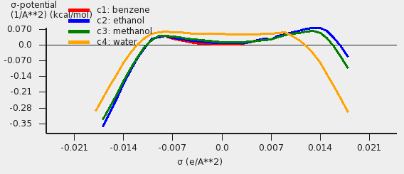
In the details for the graph window the line widths for all curves were set to ‘3’.
Note that the \(\sigma\)-potential is not calculated for values of the COSMO charge density that are non-existent on the COSMO surface of a certain compound.

| [1] | (1, 2) A. Klamt, V. Jonas, T. Bürger and J.C. Lohrenz, Refinement and Parametrization of COSMO-RS. J. Phys. Chem. A 102, 5074 (1998) |